how to make assignment excel sheet

Schedule a Demo

How to make an assignment sheet in excel.

Too many steps?

Try sourcetable..

Creating an assignment sheet in Excel can streamline the management of tasks and deadlines. This guide provides step-by-step instructions to efficiently organize your assignments within Excel's versatile framework.

While Excel is a powerful tool, we'll also explore why Sourcetable presents a more user-friendly alternative for assignment sheet creation.

Creating an Assignment Sheet in Excel

Semester assignment spreadsheet overview.

A Semester Assignment Spreadsheet is an essential tool for students to list all assignments, due dates, class information, tuition deadlines, and administrative tasks. Its one-page format allows for easy tracking of progress, helping students stay motivated and productive.

Color-Coded Excel Sheet Creation

Excel's color-coding feature enhances the visual appeal and organization of the assignment sheet. Begin with color coding, then record assignments, add more colors, organize by due date, and utilize the sheet effectively for tracking and prioritization.

Steps to Make an Assignment Tracker

Start by compiling syllabi from all classes. Use Excel to create a comprehensive Semester Assignment Spreadsheet that combines due dates with important class information. This tool is excellent for prioritizing tasks and keeping track of grades. Print out the spreadsheet for convenient access and management.

Common Use Cases

Excel vs. sourcetable: a comparative analysis.

Discover the strengths of Sourcetable, a modern spreadsheet tool designed to integrate numerous data sources seamlessly. Experience the ease of data management with its intuitive spreadsheet-like interface.

Explore the innovative AI copilot feature of Sourcetable, a game-changer in spreadsheet technology, offering real-time assistance in formula creation and template design, simplifying complex tasks.

Understand the versatility of Excel, a widely used application with robust functionalities for diverse data analysis and complex calculations, suitable for traditional spreadsheet users.

Assess the utility of Sourcetable for businesses seeking centralized data solutions, with its advanced data aggregation capabilities, versus Excel's conventional data handling approach.

Consider the efficiency gains with Sourcetable's AI-powered chat interface that streamlines formula generation and template customization, contrasting with Excel's manual formula setup.

No guides needed. Ask Sourcetable AI

Recommended How To Guides

• How to... Make A Salary Sheet In Excel
• How to... Create A Project Plan In Excel
• How to... Build A Report In Excel
• How to... Create A Workflow In Excel

Start working with Live Data

Analyze data, automate reports and create live dashboards for all your business applications, without code. get unlimited access free for 14 days..

Templates for college and university assignments

Include customizable templates in your college toolbox. stay focused on your studies and leave the assignment structuring to tried and true layout templates for all kinds of papers, reports, and more..

Keep your college toolbox stocked with easy-to-use templates

Work smarter with higher-ed helpers from our college tools collection. Presentations are on point from start to finish when you start your project using a designer-created template; you'll be sure to catch and keep your professor's attention. Staying on track semester after semester takes work, but that work gets a little easier when you take control of your scheduling, list making, and planning by using trackers and planners that bring you joy. Learning good habits in college will serve you well into your professional life after graduation, so don't reinvent the wheel—use what is known to work!

WORD & 1DER

• Jul 26, 2022

5 Easy Steps to Do the Famous Excel Assignment Sheet

Updated: May 22, 2023

Keeping up with the college schedule can be hard, especially when your university, like mine, works on a quarter system.

At the beginning of my first year, I thought using a calendar/agenda and pen would work just as great as it did in high school, but I quickly realized that most professors give out all assignments at the beginning of the term and don't remind you before the deadline. I was overwhelmed with so many assignments that I barely had time to study; everything was pilling up.

One of my roommates said that she stayed organized with a color-coded excel sheet for all assignments of the term. I later noticed that it was a trend for people to use this method, however, when I asked my friends about it, most of them wanted to do it but didn't know how to.

I had to learn how to do it myself and ended up using it for my entire freshman year. So far, it has worked wonderfully, so I figured I would share how to do it so everyone can give it a try.

Step 1. Color Coding

In this 1st step, you will decide which colors you'll be using for each subject.

Here, for example, I have my six classes abbreviated, and I colored each one differently: Linguistics is orange, Techniques of Speaking is blue and so on...

Step 2. Writing Down the Assignments

Every university has their own system regarding how assignments are given out, for example, Drexel University uses a syllabus system. Each professor will hand out a syllabus for their class at the beginning of the year, where inside, the student can find all the deadlines and assignments for the term.

Write down all the details of each assignment in the excel sheet. Add the class name, the # of the week in which it is due, the complete due date, the name of the assignment, and the status (blank or done) **more on this later.

Repeat this step for each class.

Step 3. Adding Color

This step is very simple. Select all the cells for each subject and add the color you decided on for that class. Here is how mine looks so far:

Step 4. Organizing by Due Date

To organize our sheet by due date, we must sort *custom sort* the entire chart.

Select the entire chart, every column and every line. All the assignments, no matter the class.

Right click and select *sort* - *custom sort*.

Clicking on *custom sort* must have opened the sort window.

There, you'll see a list that says column, sort by. column A. You must click on the list and change the column to the column in which your due dates are listed on.

For example: my due dates are on column D, so I change the list that says "column A" to "column D."

Next, there's a list that says sort on, values. This will remain the same so leave it at "values."

The last list says order, oldest to newest. This will also remain the same. **If yours says something different, simply click on the list and a drop down menu will pop up where you can select the option "oldest to newest."

When your "sort" window looks like this, click on *ok* to make the changes. It will organize your assignments by due date and not by class.

Step 5. Using It

The final step is to use your excel sheet, and every time you have completed an assignment, on the column status write the word "done."

"done" means you have finished the assignment.

Then, once you have turned in the assignment, you can cross off the entire line.

How to cross something of:

Shortcut in Windows computer: select the cells you want to cross off, then click Ctrl + 5.

Shortcut in Mac computer: select the cells you want to cross off, then click Command + Shift + X.

Normal way in any computer: select the cells you want to cross off, then click on the bottom right corner of the "font" section.

Once the "format cells" window has opened on the "font" section, select the *strikethrough* option under "effects."

Then click on *ok* to make the changes.

After a while of using your chart, it will start looking like this.

Make sure to add any new assignments to the chart by simply inserting a new line, changing its color and organizing it by due date. Simply repeat the 5 steps.

I hope this was helpful to keep up with your college schedule. Thank me later ;)

I appreciate your feedback. If you have any questions, concerns, and/or comments, please write them below in the comments section and I will make sure to reply to as many as I can. Have a wonderful day.

Related Posts

From Mexico to The US for College

College Packing List-the one I used

Is There Such a Thing as an Uncomplicated College Abroad Application? With This Guide, There Is

Thanks for sharing valuable insights! Your input was really helpful. I appreciate your effort and knowledge. Our top-notch Excel assignment help services are here to unlock your full potential. Whether you're struggling with complex functions or need help with data analysis, our expert team offers personalized support. Get the assistance you need to excel in your Microsoft Excel assignments and succeed academically.

• PRO Courses Guides New Tech Help Pro Expert Videos About wikiHow Pro Upgrade Sign In
• EDIT Edit this Article
• EXPLORE Tech Help Pro About Us Random Article Quizzes Request a New Article Community Dashboard This Or That Game Popular Categories Arts and Entertainment Artwork Books Movies Computers and Electronics Computers Phone Skills Technology Hacks Health Men's Health Mental Health Women's Health Relationships Dating Love Relationship Issues Hobbies and Crafts Crafts Drawing Games Education & Communication Communication Skills Personal Development Studying Personal Care and Style Fashion Hair Care Personal Hygiene Youth Personal Care School Stuff Dating All Categories Arts and Entertainment Finance and Business Home and Garden Relationship Quizzes Cars & Other Vehicles Food and Entertaining Personal Care and Style Sports and Fitness Computers and Electronics Health Pets and Animals Travel Education & Communication Hobbies and Crafts Philosophy and Religion Work World Family Life Holidays and Traditions Relationships Youth
• Browse Articles
• Learn Something New
• Quizzes Hot
• This Or That Game
• Train Your Brain
• Explore More
• Support wikiHow
• About wikiHow
• Log in / Sign up
• Computers and Electronics
• Spreadsheets
• Microsoft Excel

Create a Gradebook on Microsoft Excel: Make a Weighted Points Grade Sheet

A simple way to record your students’ grades

Last Updated: September 27, 2023 Fact Checked

Create a New Workbook

Create the layout, calculate grades with formulas, assign letter grades, weight assignments, expert q&a, things you'll need.

This article was co-authored by wikiHow staff writer, Kyle Smith . Kyle Smith is a wikiHow Technology Writer, learning and sharing information about the latest technology. He has presented his research at multiple engineering conferences and is the writer and editor of hundreds of online electronics repair guides. Kyle received a BS in Industrial Engineering from Cal Poly, San Luis Obispo. This article has been fact-checked, ensuring the accuracy of any cited facts and confirming the authority of its sources. This article has been viewed 232,859 times. Learn more...

Microsoft Excel is a great program for creating simple grade books! Using a spreadsheet (and a couple formulas) will reduce the time it takes to record and calculate grades. You don’t need to be familiar with Excel to follow our quickstart guide. This wikiHow article will walkthrough how to create a point-based grade book on Microsoft Excel.

Things You Should Know

• Create columns for student names, assignment grades, total points, possible points, numeric grade, and letter grade.
• Use the SUM function to add each student’s assignment points, then use the “/” division operator to divide their total earned points by the total possible points.
• Weight assignments by assigning more or less points.

• Alternatively, there are free templates for grade books online! Click More templates on the home page to search for “grade book” templates. You may see different templates depending on what version of Excel you’re using.
• The web app version of Excel has two grade book templates, one for points-based grading and another for percentage-based grading.

• For more general spreadsheet info, check out our guide on making a spreadsheet in Excel .

• Double click "Sheet1" at the bottom window. "Sheet1" should be highlighted.
• Type a name for the sheet. For example, “Section 1.”
• Press Enter .

• Click cell A1 to select it.
• Type the instructor’s name and press Enter . This will move your selection to A2.
• Type the class name in A3. For example, “World Geography.”
• Type the section number and meeting time in A4.
• Enter the term in A5. For example, “Fall 2022”

• This guide will cover one way to arrange your grade book. However, there are infinite ways to format an Excel spreadsheet . Try different templates and formats to find what works best for you!

• Select A7 and type “Student Number.” Row 7 will contain the column headers for each type of information you have in your grade book.
• Select A8 and type the number 1. Press Enter to enter the number in the cell and move down one.
• Type the number 2 in A9.
• Click and drag the cursor from A8 to A9. Both cells should be highlighted with a box around them.
• Hover your cursor over the lower right corner of the box until the cursor becomes a plus + (this is called the fill handle).
• Click and drag until you have a list of numbers for each student in your section.

• Select B7 and type the column header “First Name.”
• Select C7 and type the column header “Last Name.”
• Type in the students’ first and last names in columns B and C.

• You’ll insert the students’ assignment grades under each column.
• Note: For this guide, we’ll use a point-based grading structure, meaning each assignment is worth a certain amount of points.

• Note: Make sure to check your spreadsheet calculations by doing a few calculations by hand. This is a great way to catch any errors in your spreadsheet.
• Read more about the SUM function in our complete guide.

• Alternatively, you can type in the range instead.
• For example, if you have 5 assignments in columns D through H and the student names start on row 8, you’ll enter D8:H8

• Select the cell with the total summation formula. Click and drag the fill handle (the square in the bottom-right of the selection) down to the last student to automatically apply the sum formula to each row.
• Using our earlier five-assignment example, let’s say there are 10 students. The second student summation should now have a range of D9:H9, the third student D10:H10, down to the last student with D17:H17.

• Enter the possible points in each cell below the header.
• For example, if each assignment is out of 10 points, and there are five assignments, the possible points will be 50.

• The “/” symbol will divide the total cell by the possible points cell, giving you the student’s grade as a value under 1.
• For example, if a student earned 45 total points out of 50 possible points, their grade will be 0.90 (90 percent).

• You can change the grades to percentages by selecting the grade values and changing the data type to “percentage.” Find this by navigating to Fields tab > Properties group > Data Type .

• Compare the student’s grade to your grading structure.
• Insert the letter associated with that student’s grade.
• For example, if an “A” is 89 to 100 percent and a student scores a grade of 93, place an “A” in the “letter” column.

• For example, a 20-point assignments has double the weighting of a 10-point assignment.
• To weight entire categories, make their points add to the percentage of the total grade you want the category to represent.
• For example, if your course has 100 total points and you want five quizzes to represent 20 percent of the total grade, each quiz should be worth 4 points.

• Always give your grade-book a title, by clicking on the "file" tab, choose "Save As", in the Save As window, choose a location and type a name for your document. Press "Save" when ready to save. Thanks Helpful 0 Not Helpful 0
• Refer to Excel's extensive "Help" menu when in need. It offers tools on creating statistics of data. Thanks Helpful 0 Not Helpful 0
• To find out what operating system your PC has, press "Start", right click on "Computer", scroll down and click on "Properties", a system dialog box will appear with basic information about your computer. Thanks Helpful 0 Not Helpful 0

• Be sure to confirm that the equations you created for your grade book are calculating correctly. Thanks Helpful 4 Not Helpful 1
• Make sure you save your progress throughout to prevent losing information as you work. Thanks Helpful 2 Not Helpful 1
• Always save a backup of your grade book and maintain hard copies. Thanks Helpful 1 Not Helpful 2
• Computer with Windows 7, XP, or Vista
• Microsoft Office Excel 2010

You Might Also Like

About This Article

• Send fan mail to authors

Is this article up to date?

Featured Articles

Trending Articles

Watch Articles

• Terms of Use
• Privacy Policy
• Do Not Sell or Share My Info
• Not Selling Info

wikiHow Tech Help Pro:

Level up your tech skills and stay ahead of the curve

Tutorial Playlist

Excel tutorial, your one-stop solution to know about excel worksheets, your one-stop solution for excel userforms.

The Best Guide on How to Send an Email in Excel

Your One-Stop Solution That Will Help You Learn How to Convert PDF to Excel

A One-Stop Solution for Acing the Excel MIS Report

All you need to know about barcode in excel, your one-stop solution to learn mail-merge in excel and its implementation, a comprehensive guide on excel flash fill, slicers in excel: the ultimate guide to help you design and develop excel slicers, one-stop solution to learn everything about excel budget template, all you need to learn about match function in excel and its real-time implementation, everything you need to learn on how to create a pivot table from multiple sheets, the major fundamentals about xlookup in excel along with practical examples, the ultimate guide to learn how to compare two columns in excel, the best guide and your one-stop solution to master the fill series in excel, what is the date function in excel and how to implement it, your one-stop solution to designing and implementing hyperlinks in excel, one-stop solution to master everything you need to know about auto-sum in excel, dax in excel: the complete guide for dax functions and formulas in excel, a perfect guide for all you need to know about data formatting in excel, the perfect guide to learn how to add columns in excel, the perfect guide that will explain to you how to remove page break in excel, the perfect guide to explain to you how to remove blank rows in excel, the perfect guide to learning how to highlight duplicates in excel, one-stop solution understand the fundamentals of indirect function in excel, an ultimate guide to learn and implement sumifs in excel with practical examples, an ultimate guide to learning datedif in excel, an ultimate guide you need to learn about how to recover an unsaved excel file, the ultimate guide to learn and implement pivot charts in excel, learn the quickest keyboard shortcut to add dates in excel, learn how to how to group rows in excel in the easiest way, the simplest way to understand how to count colored cells in excel, how to calculate percentage in excel[with examples], how to use excel ranking function like a pro, formula for irr in excel, standard deviation in excel: a complete guide, how to create an excel worksheet: step by step guide.

Lesson 1 of 36 By Ravikiran A S

Table of Contents

Microsoft Excel is a software product designed and developed to store, organize and manipulate structured data. Excel Worksheet plays a vital role in offering multiple functionalities to ease the tedious process of managing data.

What is an Excel Worksheet?

An Excel worksheet is a software program/document that collects rows and columns designed to store information in an organized manner. An Excel worksheet also enables users to apply mathematical and statistical logic to the data and manipulate it according to the requirements of the business strategies.

So, this was a brief introduction to Excel Worksheet. In the next section, you will learn how to create a new Excel Worksheet.

Become The Highest-Paid Business Analysis Expert

How to Create an Excel Worksheet?

To create a new Excel worksheet, you need to follow the steps mentioned below.

By default, when you start Microsoft Excel, there is an option of selecting a variety of worksheets, as shown below.

You can select the option based on the requirements. For now, create a blank worksheet. The blank worksheet looks as shown below.

Insert a New Excel Worksheet

There might be a situation where you would need to include another worksheet along the side of the existing worksheet. This collection of Excel Worksheets is called an Excel Workbook. To insert a new worksheet, you can right-click on the sheet name in the bottom sheet tracker tray, as shown below.

By selecting the new worksheet option from the available options, you can create a new worksheet as displayed below.

A new dialogue box will appear on the screen, where you can select the option to include a new sheet.

In the next part, you will learn how to rename a worksheet.

Rename Excel Worksheet

You can rename the Excel Worksheet by right-clicking on the sheet name and selecting the rename option from the dialogue box as shown below.

In the next segment, you will learn how to delete a worksheet.

Delete Excel Worksheet

If you wish to eliminate the Excel Worksheet, you must right-click onto the worksheet tab and select the delete option from the dialogue box as shown below.

Worksheets in Excel can also be hidden. Now, you will see how that can be done.

Future-Proof Your AI/ML Career: Top Dos and Don'ts

Hide Excel Worksheet

Sometimes, you might have to keep a particular worksheet hidden. You can achieve this by right-clicking the worksheet name on the worksheet tray and selecting the hide option from the dialogue box, as shown below.

If you want to unhide the hidden worksheet, you can right-click on the existing worksheet and choose the option of Unhide, as shown below.

The following dialogue box will show the list of hidden sheets, and you can choose the sheet you wish to unhide, as shown below.

In the next part, you will learn to move or copy an Excel Worksheet

Move or Copy an Excel Worksheet

To move or copy an excel worksheet, you must right-click on the sheet name you wish to move or copy and select the option of copy or move option from the dialogue box as shown below.

After selecting the option, you will find a new dialogue box, as shown below.

The first step is to select the workbook where you want to copy or move the current worksheet. It can be the current workbook or a different workbook, as shown below.

The next step is to select if you want to move (cut and paste) the worksheet or copy the worksheet. If you wish to copy the sheet, then make sure you select the tick option as shown below.

If you wish to move the worksheet to a new workbook, then select the new workbook option in the first menu and do not select the tick in the last option that reads "make a copy".

In the upcoming part, you will learn to protect the cells in the excel worksheet.

Protect Cells in Excel Worksheet

To protect the cells in the Excel Worksheet, you should right-click on the sheet and select the safeguard cells option on the dialogue box, as shown below.

The following dialogue box will help you select the contents on the sheet with a password, as shown below. 

With this, you have come to an end of this "Excel Worksheet" article. 

" UserForms in Excel " can be your next stop. Generating a user form in excel will help you simplify the process to insert, delete, and manipulate data in Excel Worksheet.

Are you looking to go deeper with your Microsoft Excel learning Perhaps you are interested in furthering your career in Business Analytics?

If the answer is yes to either or both the above questions, the  Business Analytics certification course offered by Simplilearn is something you should definitely explore. This applied training program is designed to help you grasp the basic concepts of data analysis and statistics which can help you devise insights from the data available to present the findings as visualizations with the help of executive-level dashboards. You will learn all this and more in our cutting-edge program. Take a look and enroll now.

Have you got any questions for us on this Excel Worksheet tutorial? If yes, do feel free to share them in the comments section below. Our subject matter experts will resolve them for you as soon as possible.

1. What is an Excel worksheet?

You can sort and analyze raw data on excel. It is a collection of rows and columns. Each worksheet has 1048576 rows and 16384 columns. 

2. What are the basic Excel functions? 

Most basic and essential Excel functions are as follows: 

1. =IF(logical test, value if true, value if false)

=SUMIFS(sum range, criteria range 1, criteria 1, …)

3. COUNTIFS

=COUNTIFS(criteria range 1, criteria 1, …)

=TRIM(text)

5. CONCATENATE

=CONCATENATE(text1, text2, text3, …)

6. LEFT/RIGHT

=LEFT(text, num chars)

=RIGHT(text, num chars)

=VLOOKUP(lookup value, table array, column index number, range lookup)

=IFERROR(VLOOKUP(B2,$G$2:$H$12,2,FALSE),"Name not found. Check both lists")

=VALUE(text)

10. UNIQUE 

=UNIQUE(array, by col, exactly once)

3. How many worksheets are there in Excel?

In one workbook you can add 255 separate sheets. 

4. What are Excel files called?

Excel has worksheets or spreadsheets where we usually work.These worksheets are stored in a workbook. One book can have multiple worksheets in it.

5. What are the shortcut keys for Excel?

Some common shortcut keys for excel are as follows: 

• Close a workbook - Ctrl+W
• Open a workbook - Ctrl+O
• Go to the Home tab - Alt+H
• Save a workbook - Ctrl+S
• Copy selection - Ctrl+C
• Paste selection - Ctrl+V 
• Undo recent action - Ctrl+Z 
• Remove cell contents - Delete 
• Choose a fill color - Alt+H, H 
• Cut selection - Ctrl+X 
• Go to the Insert tab - Alt+N 
• Apply bold formatting - Ctrl+B 
• Center align cell contents - Alt+H, A, C 
• Go to the Page Layout tab - Alt+P 
• Go to the Data tab - Alt+A

Find our Data Analyst Online Bootcamp in top cities:

About the author.

Ravikiran A S works with Simplilearn as a Research Analyst. He an enthusiastic geek always in the hunt to learn the latest technologies. He is proficient with Java Programming Language, Big Data, and powerful Big Data Frameworks like Apache Hadoop and Apache Spark.

Recommended Resources

The Ultimate Guide to Creating Chatbots

Create and Manage Workbooks and Worksheets: Excel 2013

How To Become a Pro MERN Stack Developer in 2024

A Guide on How to Become a Site Reliability Engineer (SRE)

• PMP, PMI, PMBOK, CAPM, PgMP, PfMP, ACP, PBA, RMP, SP, and OPM3 are registered marks of the Project Management Institute, Inc.

Practice And Learn Excel Online For Free

Welcome to Excel Practice Online!

Now you can practice Excel everywhere! You can even practice on your mobile phone!

Every function and tool has an explanation followed by an online excel exercise which can be solved within the page itself, no need to download anything – All thanks to the amazing powers of Excel Online!

The tutorials are sorted from beginner level to advanced level. If you like this site please share it with your friends! 🙂

Tip for mobile phone users – tap twice on the cell you want to edit in order to edit it.

• Free Excel Courses and Resources
• Excel Self-Assessment Tool
• Free Excel Online Exercises
• Excel Basics – Zero to Hero
• Excel Tests
• Top 10 formulas and functions in Excel
• Vlookup – Tutorial with Example and Exercise Sheet
• Pivot Tables Tutorial
• Excel Shortcuts – Windows and Mac
• HOT! – Excel Mortgage Calculator – Calculate your mortgage payments and get the payment schedule for the entire period of the loan – Step-by-step tutorial on how to build a Mortgage Calculator in Excel.
• New! Excel Online Cheat Sheet – A Quick Guide To Excel’s Web Version
• Can’t find what you’re looking for? Suggest a tutorial here!
• Excel Basics – Start here if you are new to Excel! Learn how Excel works, how to perform basic calculations, and how to use cell references to save time and increase efficiency!
• Addition (Plus)
• Subtraction (Minus)
• Multiplication
• Excel Shortcuts for Windows – Master Excel Shortcuts to save time and increase efficiency!
• Excel Shortcuts for Mac – Learn how to make the most of Excel on your Mac!

Formulas/Functions

• SUM function – Sum multiple values in Excel
• MAX – find the maximum value in a range
• MIN – find the minimum value in a range
• COUNT – Count numeric values in a range
• COUNTA – Count numeric and textual values
• AVERAGE – Calculate average of a range
• Filtering in Excel – Learn how to filter your data using Excel’s Filter Tool
• Excel Sort – Learn how to sort your data in Excel.
• Flash Fill – Excel’s hidden gem for auto-completing data based on a pattern
• Remove Duplicates – Remove duplicate values in a single column or multiple columns!

Intermediate

Conditional.

• IF function – check if a condition is met
• NESTED IF – Multiple if conditions
• Conditional Formatting – Format Excel Cells based on criteria
• COUNTIF – Count cells in range which meet a certain criteria
• SUMIF – Sum range based on criteria
• AVERAGEIF – Calculate the average of a range based on criteria
• SUMIFS – Sum cells using multiple criteria
• COUNTIFS – Count cells using multiple criteria
• MAXIFS – Find maximum value in a range based on criteria
• MINIFS – Find minimum value in a range based on criteria
• AND/OR – Check if multiple criteria are met (Works great when combined with an IF function!)
• ISBLANK – Check if a cell is blank or not
• VLOOKUP – lookup value and return corresponding value from a table
• HLOOKUP – lookup value and return corresponding value from a table
• Hot!!! XLOOKUP – Excel’s next generation lookup function which combines the best features from VLOOKUP, INDEX MATCH, HLOOKUP and IFERROR/IFNA

Pivot tables

• Pivot Table – Quickly Analyze and Summarize your data using Excel’s most powerful tool!

Text Formulas

• LEFT, MID, RIGHT – Basic Text Functions
• HOT! – TEXTBEFORE & TEXTAFTER – Extract text before or after a delimiter using Excel’s brand new powerful functions!
• HOT! – TEXTSPLIT – Split your text into multiple cells using this super powerful new function!
• TEXTJOIN – Easily combine multiple cells using delimiter
• CONCAT – Combine range of cells without delimiter
• CONCATENATE – Combine two cells or more into one cell
• LEN – Find the length of a cell
• FIND – Find the position of a text within another text (Case-sensitive)
• SEARCH – Find the position of a text within another text (Case-insensitive)
• SUBSTITUTE – Replace text with another text in a cell/expression
• TRIM – Remove extra spaces from the text
• LOWER, UPPER, PROPER – Convert text to lowercase, uppercase and proper case
• VALUE – Convert data stored as text into values
• TEXT – Convert and format numbers into text
• Text to Columns – Quickly split a column into multiple columns using a delimiter. Bonus – Quickly change date formats or convert text to numbers!
• FORMULATEXT – display a formula in another cell as text

Date functions

• DAY, MONTH, YEAR – Extract day, month and year from a date in Excel
• DATE – Create a date from individual values
• WEEKDAY – Return the number of the day of the week
• EOMONTH – Return the date of the last day of the month based on a specific date

Index & Match lookup

• INDEX – Retrieve cell in nth position in a range
• MATCH – Find position of value in a range
• INDEX MATCH – Just like VLOOKUP, only better.

Other advanced tools

• SUMPRODUCT – Sum the products of Excel ranges
• Excel Wildcards – Advanced searching and matching in Excel
• Advanced Filter – Filter by multiple criteria in the same column, or even in different columns!

Power Query

• Combine data from multiple Excel workbooks using Power Query
• Column from Examples tool – Learn the secret to mastering Power Query without any prior knowledge!
• Unpivot columns easily using Power Query

Secret Excel Functions

This section covers Excel functions that are not available in most of Excel’s versions. These functions will unlock a new set of capabilities such as fining only unique values, sorting, and filtering – the tutorials below will help you with mastering Excel’s new functions!

• UNIQUE – Extract unique values from a range
• SORT Function – Sort range dynamically
• SORTBY – Sort range dynamically by using another range
• FILTER Function – Filter range by specific criteria
• RANDARRAY – Create an array of random numbers 
• SEQUENCE – Create a range of sequential values
• LET – Assign values and calculations to names to improve your formula’s ease of use, readability, and performance!
• HOT! – LAMBDA – The mother of all functions that will help you create amazing and powerful custom functions for your own need! 
• VSTACK – Vertically stack arrays/ranges in Excel
• HSTACK – Horizontally stack arrays/ranges in Excel
• CHOOSEROWS – Return specific rows from a range or array
• CHOOSECOLS – Return specific columns from a range or array
• TOROW – Convert a range/array into a single row
• TOCOL – Convert a range/array into a single column

Financial Functions

Learn how to use Excel to make financial calculations!

• Excel Financial Calculator – quickly calculate PV, FV, PMT, NPV, IRR
• PMT – Calculate the periodic payment amount of a loan, mortgage, or another financial instrument
• PPMT & IPMT – Find the Principal and Interest portion of a certain payment
• PV – Find the Present Value of a loan, mortgage, or any other financial instrument 

Excel Macros – VBA (Visual Basic for Applications)

• Start here – How to run your first VBA Macro in Excel without knowing VBA? 

Excel Data Sheets for Practice

Want to do some freestyle practice? Create your own Excel playground with our blank excel Worksheet!

• Excel-Online Blank Worksheet
• Excel Practice Data

How to Calculate in Excel – Excel-Online Calculators

• How to Calculate GPA in Excel
• How to Calculate BMI in Excel
• How to Calculate Density in Excel
• How to Calculate Weighted Average in Excel

Terms and Conditions - Privacy Policy

Homework To Do List

A spreadsheet can be a useful tool for tracking your homework assignments, due dates, and completion status. The homework list template on this page was designed based on my original To Do List Template for Excel. I simplified it a bit for and modified it specifically for tracking homework assignments. You can download the Excel file or the blank printable PDF version if all you need is a blank form to use for your student planner.

Homework To Do List Template

License : Private Use (not for distribution or resale)

"No installation, no macros - just a simple spreadsheet" - by Jon Wittwer

Description

Drop-Down Lists for Status and Priority - The Status column lets you choose from "Not Started", "Incomplete", "In Progress", and "Complete." The Priority columns lets you choose between "High", "Medium", or "Low." If you want to edit the items in the drop-down lists, just select the cells you want to edit and go to Data > Data Validation and edit the comma-delimited lists.

Conditional Formatting for Priority and Due Date - I've set up the Priority column to show "High" as a bold red font and "Low" as a blue font. The Due Date uses icon sets to show when the date is past due. If you need or want to edit these rules, go to Home > Conditional Formatting > Manage Rules and select "This Worksheet" from the drop-down to see all the rules for the worksheet.

A Worksheet for Each Class - You can duplicate the main worksheet tab to create a homework list for each of your classes. Just right-click on the worksheet tab and select "Move or Copy" and check the "Create a copy" box. Then you can rename the tabs "ENG 101", "MATH 101" etc.

Completed Assignments - When you select "Complete" from the Status column, the font in that row will change to a gray strikethrough . You can edit the conditional format rule to change that if you want.

Printable Homework List

• Create a Drop Down List in Excel at vertex42.com - Explains how you can create a drop-down list like the one used in the Priority column.

Follow Us On ...

Related templates.

Education Templates

Excel Tutorial: How To Organize Assignments In Excel

Introduction.

When it comes to managing assignments, Excel can be a powerful tool to keep everything organized and easily accessible. Whether you're a student, a teacher, or a project manager, using Excel for assignments can help streamline your workflow and increase productivity.

Excel provides a range of features for organizing, sorting, and analyzing data, making it an ideal platform for managing assignments of all kinds. This tutorial will guide you through the process of setting up an Excel spreadsheet to effectively manage and track assignments, helping you stay on top of deadlines and priorities.

Key Takeaways

• Excel is a powerful tool for managing assignments and increasing productivity for students, teachers, and project managers.
• Understanding the basics of Excel, including the layout and functions, is essential for effective assignment organization.
• Creating a new spreadsheet and inputting data with proper formatting sets the foundation for organized assignment management.
• Utilizing formulas, functions, and visual enhancements such as color-coding and charts can further enhance assignment organization in Excel.
• By practicing and implementing the tips provided in this tutorial, users can effectively track deadlines and priorities in Excel, ultimately improving their workflow.

Understanding Excel Basics

When it comes to organizing assignments in Excel, it is important to have a good understanding of the basics of the software. This will ensure that you are able to utilize its features effectively and efficiently. In this chapter, we will explore the layout of an Excel spreadsheet, the different tabs and their functions, and provide some tips for navigating and selecting cells in Excel.

Rows and Columns

An Excel spreadsheet is made up of rows and columns. The rows are denoted by numbers and the columns are denoted by letters. This creates a grid structure that allows for easy organization of data.

Each intersection of a row and column is referred to as a cell. This is where you will input your data, formulas, and other information.

An Excel file can consist of multiple worksheets, each of which contains its own grid of cells. This allows you to organize different sets of data within the same file.

The Home tab contains the most commonly used commands for formatting and manipulating data, such as changing fonts, aligning text, and applying borders.

The Insert tab allows you to add various elements to your spreadsheet, such as tables, charts, shapes, and hyperlinks.

Formulas Tab

The Formulas tab is where you can find all the functions and formulas that Excel offers, allowing you to perform calculations and manipulate data.

The Data tab provides tools for sorting and filtering data, as well as importing and exporting data from external sources.

The Review tab contains tools for proofreading and collaborating on your spreadsheet, such as spell check, comments, and protection.

The View tab allows you to customize the way your spreadsheet is displayed, such as adjusting zoom, freezing panes, and showing or hiding gridlines.

Keyboard Shortcuts

Learning keyboard shortcuts can greatly improve your efficiency in Excel. For example, pressing Ctrl + Home will take you to the first cell of the spreadsheet, while Ctrl + Shift + Arrow Key will allow you to quickly select a range of cells.

Using the Name Box

The Name Box, located next to the formula bar, displays the name of the selected cell or range of cells. You can use this to quickly navigate to a specific cell by entering its reference in the Name Box.

Mouse Navigation

Clicking on a cell will select it, and clicking and dragging will allow you to select a range of cells. You can also use the scroll bars to navigate around the spreadsheet.

Creating a New Spreadsheet

When it comes to organizing assignments in Excel, the first step is to create a new spreadsheet. This can be done by following a few simple steps.

To open a new Excel workbook, start by opening Microsoft Excel on your computer. Once the program is open, you can either click on "File" in the top left corner and select "New" to create a new workbook or use the keyboard shortcut Ctrl + N. This will open a new blank spreadsheet for you to work with.

Formatting Options:

• Adjusting column width and row height to accommodate data
• Applying cell borders and shading for better visual organization
• Using formatting tools for fonts, colors, and text alignment

Once the new spreadsheet is open and formatted to your preference, it's time to input the assignment data.

• Start by selecting the cell where you want to input the data
• Type the assignment details, such as the assignment name, due date, and any other relevant information
• Continue inputting data into subsequent cells for each assignment

Organizing Assignment Data

When managing multiple assignments in Excel, it's essential to keep the data organized for easy access and reference. By utilizing the following methods, you can streamline your workflow and stay on top of your tasks effectively.

A. Use of headers and subheaders for assignment details

When creating your assignment spreadsheet, it's crucial to use clear and descriptive headers to outline the assignment details. This includes task name , due date , subject , priority level , and any other relevant information. By using subheaders, you can further categorize specific details within each assignment, such as subtasks , additional notes , or attached files .

B. Examples of how to categorize assignments

Excel offers various ways to categorize assignments, making it easier to manage and prioritize your workload. You can categorize assignments by due date , subject , or priority level by creating separate columns for each category. For example, you can use the due date column to sort assignments by their deadline, the subject column to group assignments by course or project, and the priority level column to identify urgent tasks.

C. Benefits of using filters and sort functions

Utilizing Excel's filter and sort functions can greatly enhance the organization of your assignments. By applying filters, you can quickly narrow down specific assignments based on criteria such as subject or priority level . The sort function allows you to arrange assignments in ascending or descending order based on the due date or any other relevant category, providing a clear overview of your upcoming tasks.

Using Formulas and Functions

One of the key features of Excel is its ability to perform calculations and automate processes using formulas and functions. In the context of organizing assignments, these tools can be incredibly useful for tracking deadlines, progress, and grades.

Sum and Average:

Weighted average:, today's date:, conditional formatting:, progress tracker:, deadline reminders:, adding visual enhancements.

Visual enhancements can help make your Excel spreadsheet more engaging and easier to navigate. Here are some tips for adding visual elements to your assignment organization:

Formatting options such as bolding, italicizing, and underlining can help draw attention to important information in your spreadsheet. Additionally, adjusting font styles and sizes can help make your spreadsheet more visually appealing and easier to read.

Color-coding can be a powerful tool for visually organizing your assignments. By assigning different colors to different categories or priorities, you can quickly identify and differentiate between various tasks. Conditional formatting, on the other hand, allows you to automatically apply formatting based on specific criteria, making it easier to highlight important data or trends.

Charts and graphs can help provide a visual representation of your assignment data, making it easier to identify patterns, trends, and discrepancies. Consider using pie charts, bar graphs, or line graphs to effectively communicate your assignment information in a visually appealing way.

In conclusion, we have discussed the key points of how to organize assignments in Excel, including using tabs and color-coding to keep track of different tasks, and utilizing formulas for automating calculations and deadlines. Excel is an invaluable tool for organizing assignments due to its flexibility, efficiency, and customization options, making it a great choice for students and professionals alike.

We highly encourage our readers to practice using Excel for their assignment organization, as it can greatly streamline their workload and improve their productivity. For those who want to further enhance their Excel skills, there are numerous online resources, tutorials, and courses available to help you master this powerful tool.

Immediate Download

MAC & PC Compatible

Free Email Support

Related aticles

The Benefits of Excel Dashboards for Data Analysts

Unlock the Power of Real-Time Data Visualization with Excel Dashboards

Unlocking the Potential of Excel's Data Dashboard

Unleashing the Benefits of a Dashboard with Maximum Impact in Excel

Exploring Data Easily and Securely: Essential Features for Excel Dashboards

Unlock the Benefits of Real-Time Dashboard Updates in Excel

Unleashing the Power of Excel Dashboards

Understanding the Benefits and Challenges of Excel Dashboard Design and Development

Leverage Your Data with Excel Dashboards

Crafting the Perfect Dashboard for Excel

An Introduction to Excel Dashboards

How to Create an Effective Excel Dashboard

• Choosing a selection results in a full page refresh.

• Contact sales

Start free trial

15 Excel Spreadsheet Templates for Tracking Tasks, Costs and Time

Still using spreadsheets to manage your projects? Revolutionize your project management with ProjectManager. Plan projects, manage resources and track progress with powerful features the whole team can use.

Excel spreadsheet templates are a great tool to track the costs, time and performance of your team. We’ve collected ProjectManager’s 15 best Excel spreadsheet templates for tracking that you can download and use for free.

1. Dashboard Template

A dashboard is how you keep track of your work, including the time spent on tasks, what you’re spending and if you’re making progress as planned. ProjectManager’s free dashboard template for Excel gives you an overview of how you’re doing on your work. This information is vital to know if you’re overspending or running behind on your schedule.

ProjectManager’s free dashboard template has several widgets that monitor metrics in your work. For example, there’s a color-coded task graph that shows if your tasks are complete, in progress, not started or overdue. There’s also a workload chart for managing teams and making sure their workload is balanced.

There’s another task graph that measures the duration of the tasks, which is helpful in seeing what’s getting done on time and what’s taking too long. Finally, there’s a cost bar chart to help you stay on budget.

This Excel dashboard template can manage your work, but it’s a static document that must be updated manually. Project tracking software automates that process. ProjectManager is better than Excel spreadsheet templates as it helps to accumulate real-time data, crunch the numbers and display it. Get started with ProjectManager free today.

Not all project management software offers the same project dashboards. ProjectManager’s project dashboard comes equipped with the right project management features to help you keep track of time, tasks, costs and more.

2. Task Tracker Template

ProjectManager’s free task tracker for Excel template can organize and keep track of your work. It’s similar to a to-do list, where you just need to add the work and manage it. Having a task list is the first step to controlling your work.

This task tracker spreadsheet captures the details of your work. Add the name of the task and include dependent tasks. You can assign it to yourself or someone on your team.

Next, set the priority and when you expect to finish. Finally, there’s a column to mark its status, which is essential to track your work. It has everything you need to track your tasks at a basic level with an Excel spreadsheet.

3. Budget Spreadsheet for Cost Tracking

Managing costs in your work is as important as meeting deadlines. ProjectManager’s free budget template for Excel helps you keep to your budget by tracking your financial details on one spreadsheet.

Tasks cost money, and the budget defines the costs of the resources you’ll employ to deliver those tasks to completion. First, the spreadsheet template has a numbered list that corresponds to your work breakdown structure (WBS) . Then, there are labor costs including planned vs. actual hours plus the cost per hour. Materials are broken down by units and cost per unit.

There’s also room for other line items on your budget, which include travel, equipment, fixed and miscellaneous costs. Finally, there are columns to collect the budgeted and actual cost for each line item, then a balance showing if the line item is above or under budget.

Related: How to Track Project Expenses

4. Timeline Template

ProjectManager’s free timeline template in Excel is perfect for scheduling your project from start to finish in Excel. It’s a way to view all your tasks and keep on schedule. You can even add milestones!

To get started with this free timeline template, you first need to list your tasks and give them a name. Each task must have a start date and an end date, plus the time you think it’ll take to complete.

You add all that data to the left side of the template, which is a normal tracking spreadsheet. Then, on the right, you’ll see the timeline that lays out your tasks as horizontal bars across a timeline. It’s easy to see how long it’ll take to complete each task.

Excel spreadsheet templates are good for beginners, but if you want to take your planning even further, upgrade to online software that lets you build timelines in minutes. ProjectManager has online project timelines that update instantly as the team collaborates on tasks. Track costs, workload, planned vs actual progress and more. Get started for free.

5. Action Plan Spreadsheet

Managing work means outlining the steps you must complete to achieve your goals. Use ProjectManager’s free action plan spreadsheet for Excel to track tasks and detail the strategy you’ll use to complete your work on time and within budget.

We’ve broken up this action plan template into three sections. The first is the action steps, which note the priority and list tasks, phases and assignments. There’s also space to note the status of your tasks and track their progress.

Section two of this Excel spreadsheet template is a timeline, with start and due dates, including planned hours. Finally, section three focuses on resources; for example, which department is responsible for which task, what materials are needed and what are the resource costs?

6. Status Report Template

Knowing where you are at any particular point in the project life cycle is how you manage time and costs. Our free status report template is a great tool to track your progress and stay on schedule.

This free status report template is made up of five sections: project information, project status summary, project health, risk management overview and a conclusion that includes recommendations for the future.

A status report is a cornerstone of tracking your work. It’s used in project management and work management alike because it gives managers a picture of their planned vs actual progress. It’s also a powerful tool when presenting to stakeholders.

7. Risk Tracking Spreadsheet

No matter how well-planned your work is, there are unknowns that can impact your progress. Use ProjectManager’s free risk register spreadsheet to help you plan for risks in your work.

This free risk register for Excel has columns to ID the risk to make it easier to track. There’s a column to describe the risk and explain how it’ll impact the work you’re doing if it goes from a risk to an actual issue .

For each risk you identify on the template, you can add a risk response, which is the response you’ll take if the risk actualizes. You can also note the risk level. Then, if you’re working in a team, you can assign the risk so that the team member is responsible for identifying and rectifying it.

8. Change Tracking Spreadsheet

Download ProjectManager’s free change tracking spreadsheet for Microsoft Excel to manage change when it impacts your work management. It’ll help you control change so it doesn’t make you spend too much overtime or incur additional costs.

A change log Excel spreadsheet is one of the most important Microsoft Excel templates we offer. It’s a spreadsheet template that captures change when it happens. You can number changes for better tracking and note when the change first came up and who discovered or requested it.

You can then prioritize the change, and you or a team member can take ownership to see it through to completion. The Excel spreadsheet tracks the change from discovery to recovery and ensures that no change order is lost in the cracks.

9. Time Tracking Spreadsheet

There’s no better template to track the time you spend on your tasks than with ProjectManager’s free time tracking spreadsheet . This timesheet is great for you or team members to record the amount of time spent on work.

This timesheet Excel spreadsheet template has space for your name or the name of the employee, their department, supervisor and hourly rate. The template collects their hours, such as their start time and end time for their workday. There’s even a place to add overtime and lunch.

Then, the total for the week is added and multiplied by the pay rate to show the total amount the employee is owed. Finally, there’s a line for the employee to sign and the supervisor to look it over and sign it, if accurate.

10. Multiple Project Tracking Template

When you’re managing a portfolio or program, you have to monitor all your projects in one place to make insightful decisions as to how to allocate resources. Using our free multiple-project tracking template for Excel gives you a high-level overview of every project for which you’re responsible.

Once you download the free Excel template, you’ll find it’s formatted with three projects, one stacked on top of the other. You can copy and paste to add as many projects as needed. You can also add columns if you need to track something not already on the template.

Each project spreadsheet allows you to list all the project tasks by name and description, as well as if they’re dependent on another task. There’s space to add who’s assigned to each task. Each task has a start and planned end date, and planned cost, with an actual end date and actual cost to help you track the project.

11. Issue Tracking Template

Issues are problems that arise while executing your project. These issues must be quickly identified and resolved to keep the project on schedule and within its budget. With our free issue-tracking template for Excel , you have the tools to monitor the progress of resolving those issues.

The free template is ideal to capture risks, which become issues if they in fact show up in your project. When they do, you already have them described in the template and what their potential impact is. Next, you can define its priority, from low to critical, which helps you determine which risks need your immediate attention.

There’s also a place to note the date the issue first was discovered and when it was closed, as well as the team member who’s responsible for resolving it. Finally, the free template states the department that’s handling the issue and there’s a column to note its status when tracking the issue.

12. To-Do List Template

Everyone has work to do, and getting that work done efficiently requires task management. At its most basic, that means having a list of your tasks. It’s the first step to getting organized. That’s where our free to-do list for Excel comes in handy.

A to-do list is a simple but highly effective tool. Simply list the tasks you’ve been assigned or you can even use it for household chores. Next, you’ll want to give each task a start and due date. This is the duration or timeframe in which you want the work completed.

Now, you’ll want to track your progress. The free to-do list template shows the percentage complete for each task. It’s a satisfying feeling to see the cell move from 25 percent to 100 percent. Then there’s a column to note the progress. Before you know it, your work is done.

13. Inventory Template

If you’re a manufacturer or have a company with which you carry stock that you need to run your business, then you need our free inventory template for Excel . Use it to prevent production delays by keeping track of what you’re warehousing.

Use this free template to record the level of your inventory and track its turnover. First, each line is numbered to make it easier to find the item you want. Then the item is listed and described, with the unit price noted and the quantity you have in stock.

Now you can calculate the inventory price, which is the unit price multiplied by the number in stock. This Excel spreadsheet template does this automatically. There’s a column to note whether you need to reorder, what level to reorder, how long it takes to restock and what that reorder quantity should be.

14. Progress Report Template

Project reports are essential for a number of reasons. One, they help you monitor your progress and performance, and two, they’re a great tool for keeping stakeholders updated. Our free progress report template for Word captures an overview of the activities and tasks that occurred over a specific period.

The free progress report is broken up into a number of different sections. There’s a summary, which provides a quick overview of what’s to follow, including pertinent data, such as the project scope, schedule, cost and risk for the time period being reported on.

Then there’s a section in this Excel spreadsheet template that goes over the tasks that have been executed over a period of time covered in the report. There’s space to note the status of tasks that aren’t yet completed and a section to list issues, talk about the budget and more. It’s a great way to capture a snapshot of the project in time.

15. Work Schedule Template

Need help managing your human resources or operations planning? Check out our free work schedule template for Excel . This free template lists all your employees and their working hours, including responsibilities, over a day, week or month.

Use the work schedule template to keep your employees productive and help with tracking your resource utilization and scheduling. You can also use it to prioritize tasks and balance your team’s workload, which leads to greater productivity and happier employees.

Our free spreadsheet template has a weekly and monthly work schedule. Both list your employees, their tasks, which project they’re working on and then their hours, either day-by-day or over the course of a month. This will help most organizations and even long-term projects.

Use ProjectManager to Track Time, Costs and Tasks Better Than Excel

Templates and Excel spreadsheets for tracking are great, but as noted, they can only do so much. ProjectManager is online work management software that connects everyone, no matter where they work, what time, department or skill level. It does so in real-time to ensure that everyone is collaborating and working on the most recent data.

Automatically Fill Out Timesheets

Take timesheets, for example. Instead of having your employee fill out the timesheet, ProjectManager’s timesheets autofill their tasks and update the time they’ve spent. This streamlines payroll but also offers a window into tracking the time they spend on their tasks. That way, you know if they’re meeting their quota. Once submitted, timesheets are locked and secure.

Work the Way That Suits You

Multiple project views allow everyone on the team to work how they want. Managers can plan ahead on Gantt charts that show all their tasks on a timeline. The duration bar that connects each task’s start and end dates automatically shows progress based on how much of it is shaded. Teams can use task lists, kanban boards or calendars if they prefer, all of which are updated and show progress. No tool is more flexible for planning and tracking work.

Generate One-Click Reports in Seconds

Tracking time, costs and more is easy with ProjectManager’s one-click reports. Get status reports, reports on tasks, timesheets, expenses and more. These reports take complicated data and turn it into insightful and easy-to-read reports to monitor progress and more. Reports can also be filtered to see only the data you want and then shared to keep stakeholders updated.

Related Excel Project Management Content

While Excel is not a project management software, it can still be a very helpful for managing various aspects of your projects. That’s why we’ve created dozens of blogs, templates and guides to help you use Excel for project management.

• Essential Excel Report Templates
• Free Manufacturing Excel Templates
• Free Excel Construction Templates
• Free Word & Excel Templates for Business
• How to Create a Project Timeline in Excel (Free Template Included)
• How to Make a Gantt Chart In Excel Step-By-Step (Template Included)
• 25 Must-Have Project Management Excel Templates and Spreadsheets

ProjectManager is award-winning project management software for teams. Our real-time tool tracks time, costs and more to ensure you’re always on schedule and never spending over your budget. Join the 35,000+ people using our software to track tasks, cost and time. Get started with ProjectManager free today.

Deliver your projects on time and on budget

Start planning your projects.

How to Make a Spreadsheet in Excel, Word, Google Sheets, and Smartsheet for Beginners

By Andy Marker | June 13, 2017

• Share on Facebook
• Share on LinkedIn

Link copied

Spreadsheets are grid-based files designed to organize information and perform calculations with scalable entries. People all around the world use spreadsheets to create tables for any personal or business need.

However, spreadsheets have grown from simple grids to powerful tools, functioning like databases or apps that perform numerous calculations on a single sheet. You can use a spreadsheet to determine your mortgage payments over time, or to help calculate the depreciation of assets and how it will affect your business’s taxes. You can also combine data between several sheets, and visualize it in color-coded tables for an at-a-glance understanding. With all the new functionality, using a spreadsheet program can be intimidating for new users.

In this article, you will learn  how to create a spreadsheet in Excel with step-by-step instructions, details on what you can do with all its main functions , information on how to navigate the tools , and some free, easy-to-use templates . You’ll also learn how to do the same for spreadsheets you can create in Word, Google Sheets, and a powerful spreadsheet application, Smartsheet.

How to Create a Spreadsheet in Excel

The world’s most robust pure spreadsheet application, Excel, comes as part of both Microsoft Office and Office 365. There are two main differences between the two offerings: First, Microsoft Office is an on-premise application whereas Office 365 is a cloud-based app suite. Second, Office is a one-time payment, and Office 365 is a monthly subscription. Excel is available for both Mac and PC.

"Spreadsheets keep you organized. Rows and columns, formatting, formulas, filtering. That's the building blocks of structure and overview." - Kasper Langmann, Co-founder of Spreadsheeto

Unique Features of Excel

With over 400 functions, Excel is more or less the most comprehensive spreadsheet option when it comes to pure calculations. It also has strong visualization abilities, including  conditional formatting, Pivot Tables, SmartArt, graphs, and charts. Home and business users alike can create powerful spreadsheets and reports to track data and inform their decisions.

One powerful Excel feature is Macro, little scripts and recordings you can create to make the program perform different actions automatically. While no other spreadsheet program has this type of feature, it is complex and can pose difficulty for beginners.

Excel also has close tie-ins with Microsoft Access, a database program, which can add power. In general, Excel integrates best with databases and any dataset requiring many calculations per workbook.

Understanding Your Main Screen

When you first open Excel in Office 365 or a newer version of Microsoft Office, you’ll see a basic screen. Here are the key features in this view:

A.  Basic App Functions: From left to right along this top green banner you’ll find icons to: reopen the Create a Workbook page; save your work; undo the last action performed and display which actions were recorded; redo a step that’s been undone; select which tools appear below.

B. Ribbon: This grey area is called the Ribbon, and contains tools for entering, manipulating, and visualizing data. There are also tabs that focus on specific features. Home is selected by default; click on the Insert , Page Layout , Formulas , Data , Review , or View tab to reveal a set of tools unique to each tab. We’ll cover this more in the “Navigating the Ribbon” section later on.

C. Spreadsheet Work Area: By default the work area is a grid. Along the top are column headers A through Z (and beyond), and along the left side are numbered row headers. Each rectangle in the spreadsheet is called a cell, and they are each named according to their column letter and row number. For example, the cell selected here is A3.

D.  Formula Bar: The Formula Bar displays the information contained within a highlighted single cell or range of cells. If in cell A1 you entered “1” as a value, “1” will appear in the Formula Bar . Plain text that you enter in a cell will also appear in the Formula Bar .

There are cases where what you see in the Formula Bar is different than what’s in the cell. For example, let’s say A1 = 1 and A2 = 2. If you create a formula in A3 that equals A1 + A2, then the A3 cell in your worksheet would show “3,” but the Formula Bar would show “=A1+A2.” This is important when you’re trying to move cells to other parts of your worksheet - remember that the display “value” of a cell isn’t necessarily what the cell contains.

That said, other formulas that reference a cell will take into account the current value of a cell. If A4 = A3 + 1, then it would be equal to 4, because it stacks the formula of A3 (A1 + A2) with A4 = A3 + 1. Formulas can reference other formulas multiple times.

E. Search Bar: Simply type the value you want to find to highlight all cells containing that value. It doesn’t have to be an exact match. For instance, if you searched for “o,” a cell labeled “Dogs” would appear among your search results.

F. Sheet Tabs: This is where the different sheets in your workbook can be found. Each sheet gets its own tab, which you can name yourself. These can be useful to separate out data so that one sheet doesn’t get too overwhelming. For example, you might have an annual budget, where each month is a column, and each row is a type of expense. Instead of keeping every single year you track on one sheet and scrolling horizontally, you can make each tab a different year containing 12 months only.

Note that data from different sheets in the same workbook can be referenced for formulas. For example, if you have two sheets, Sheet1 and Sheet2, you could bring Sheet2 data into Sheet1. If you wanted cell A1 in Sheet1 to equal the A1 in Sheet2,  you’d enter this formula into A1: “=Sheet2!A1”. The exclamation mark calls on the previous sheet referenced before locating the data.

G. Viewability Options: The left icon is Normal which shows the worksheet as it appears in the image above, and the right icon is Page Layout , which divides your worksheet into pages resembling how it would look when printed, with the option to add headers. The slider with the “-” and “+” on it is for scale or zoom-level. Drag the slider left or right to zoom in or out.

Navigating the Ribbon

The Home tab is where you manage the formatting and appearance of your sheet, along with some simple formulas you’ll always need. 

A. Copy and Paste Tools: Use these tools to quickly duplicate data and format styles in the spreadsheet. The Copy tool can either copy a selected cell or group of cells, or copy an area of the spreadsheet that you’ll use as a picture in another document. The Cut tool moves the selection of cells to a new destination rather than duplicating it. 

The Paste tool can paste anything in your clipboard into the selected cell, and typically retains everything including the value, formula, and format. However, Excel has a wealth of pasting options: you can access these by clicking the down arrow next to the Paste icon. You can paste what you’ve copied as a picture. You can also paste what you’ve copied as values only, so that instead of duplicating the formula of a copied cell, you duplicate the final value shown in the cell. 

The Format paintbrush copies everything related to the formatting of a selected cell. When you select a cell and click Format , you can then highlight a whole range of cells, and each one will take on the formatting of the original cell, without changing their values.

B. Visual Formatting Tools: Many of these tools are similar to those found in Microsoft Word. You can use the formatting tools to change the font, size, and color of typed words, and make them bold, italicized, or underlined. It also has a couple spreadsheet-specific formatting options. You can choose which sides of the cell get additional borders, and their style and thickness. You can also change the highlight color of the entire cell. This is useful for creating visually-appealing borders or differentiating rows or columns on large sheets, or for highlighting a particular cell that you want to accentuate. 

C. Position Formatting Tools: Align cell data to the top, bottom, or middle of the cell. There is also an option for angling the values displayed, which can make it easier to read. The bottom row has familiar options for left, center, and right alignment. There are also indent right and left buttons.

D. Multi-cell Formatting Features: This section contains two very important features that solve common problems for new Excel users. The first is Wrap Text . Normally, when you enter text into a cell that extends beyond the size of the cell, it spills into the next cell. For example, if you type “Budgeted Items” into A1, some of the word “Items” spills into B1. Then, if you type into B1, you cover up any characters from A1 that extended into B1. The extra text from cell A1 still exists, but now it is hidden. If you don’t want to widen the cells, click the Wrap Text icon on A1 - this will split “Budgeted Items” into two stacked lines instead of one within A1. This makes the entire row taller to accommodate the content. Now, typing into B1 won’t cover up existing text.

The other tool in this section is Merge and Center . There are instances when you may want to combine several cells and have them act as one long cell. For example, you might want a header for an entire table to be clear and easy to read. Select all the cells you want combined, click Merge , and then type your header and format it. Though the default setting for headers is centered text, simply click the drop-down arrow to select different merging and unmerging options.

E. Numbers-based Format Settings: A drop-down menu has options for number formatting. For example, currency places everything you select into “$0.00” format, and percent turns .5 or ½ into “50%”, date options. These are the basic format options, but you can select More Number Formats from the drop-down menu to get more specialty use cases (different countries’ currencies, or adding the “(xxx)xxx-xxxx” formatting to phone number sequences). Often, you may use these tools on entire columns to make all data in one category behave the same way.

F. Table or Sheet Formatting: Format as Table and Cell Styles allow you to use presets or customize tables (for example, with alternating row colors and highlighted header bars). Select your data range and choose a style to standardize formatting. 

Conditional formatting is a bit more complex. Use the drop-down menu to select from a range of options, like inserting helpful visual icons to represent status or completion, or changing the color of different rows. Most important are the conditional rules , which are created with a simple logic. For example, let’s say you have a column with data in A1 through A3, and A4 holds the sum of these three cells. You could place formatting on A4 with a rule that says “if A4 > 0, then highlight A4 green.” Then, you could add another rule that says “if A4 < 0, then highlight A4 red.” Now you have a quick visual reference where green = a positive number and red = a negative number, which will change based on what you enter into A1, A2, and A3. 

G. Row and Column Formatting Tools: The Insert drop-down menu puts cells, rows, or columns before or after a selected area on the sheet, and Delete removes them. The Format drop-down lets you change the height of rows and the width of columns. It also has options for hiding and unhiding certain sections. 

H. Miscellaneous Tools: Starting at the top left, there’s AutoSum , which allows you to select a swath of cells and place the sum in the cell located right below or directly to the right of the last selected data point. You can use the drop-down to change the function to calculate the average, display the maximum, minimum, or the count of numbers selected.

Use Fill to take a cell’s contents and extend them in any direction for as many cells as you want. If the cell contains a value, Fill will simply copy the value over and over again. If it contains a formula, it will recalculate its relative position for each new cell. If the first cell equals A1+B1, then the next would equal A2+B2, and so on. 

The Clear button lets you either clear the value, or just clear cell formatting. 

Sort & Filter tools let you choose what to display, and in what order. At the base level, this tool sorts cells containing text from A to Z, and cells containing numbers from lowest to highest. It can also sort by color or icon. Sorting and filtering helps surface only the data you need. 

Use the Insert tab to add extra elements to your Excel workbook that go beyond text and colors.

A. These tools control PivotTables , an important Excel function. Think of PivotTables as “reports,” a quick way to view all your data, analyze trends, and draw conclusions. By selecting at least two rows of data and clicking on PivotTable , you can quickly generate a visually-appealing table. Going through this process launches the PivotTable Builder , which helps you select columns to include, sort them, and drag-and-drop them to quickly construct your table. They can include collapsible rows to make reports interactive and uncluttered. There is also a button for Recommended PivotTables, which can help when you don’t know where to start.

Table builds a simple table that includes any number of columns you select. Rather than placing the table elsewhere on the worksheet, it turns the data into a table on the spot, and applies customizable color formatting.

B. This section lets you insert visual elements, like picture files, pre-built shapes, and SmartArt. You can add shapes and resize, recolor, and reposition them to create intuitive data sets and reports. SmartArt objects are prebuilt diagrams that you can insert text and information into. They’re great for representing what the data says in another place on your workbook.

C. These tools are for inserting elements from other Microsoft products, like Bing Maps, pre-built information cards about People (from Microsoft accounts only), and add-ins from their store.

D. Use these tools to create charts and graphs. Most of them work only if you select one or more data sets (numbers only, with words for headers or categories). Charts and graphs function like you’d expect - just select the data you want to visualize, then select your desired type of visual (bar charts, scatter plots, pie charts, or line graphs). Creating one will bring up formatting options where you can change the color, labels, and more.

E. Sparklines are more simplistic graphs that can fit in as little as one cell. You can place them next to data for a small, quick visual representation.

F. Slicers are big lists of buttons that make your data more interactive. You can select a PivotTable you’ve created, and then create a slicer from it - this allows a viewer to click on buttons that correlate to the data they want to filter. 

G. This hyperlink tool allows you to make a cell or table into a clickable link. Once a viewer clicks on the affected cell(s), they’ll be taken to whatever website or intranet site you select.

H. Recent versions of Excel allow for better collaboration - insert comments on any cell or range of cells to add more context. You can open or close the comments so the worksheet doesn’t get too cluttered.

I. A Text Box is useful when you’re creating a report and don’t want typed words to behave like cells. It makes it easy to move your text around, rather than cutting and pasting cells (which could potentially mess up the formatting of real data). The next area is for Headers & Footers , which will take you to the page layout view - here you can add headers and footers for the entire page. WordArt , on the other hand, lets you embellish text. Insert Object lets you place entire files (Word documents, PDFs, etc.) into the worksheet.

J. This section lets you insert Equations and Symbols .  Use equations to write a math equation with fractions, variables, and more that you can place in your sheet like a Text Box . For instance, this can be helpful for explaining how a portion of a table was calculated in a report. Symbols , on the other hand, can be inserted directly into cells, and include all non-standard characters from most languages, as well as emojis.   The Page Layout tab has everything you need to change the structural parts of your worksheet, especially for purposes of printing or presenting.

A. Use these buttons to quickly adjust the visual style of your entire sheet. You can regulate the fonts and colors, and use the Themes section to quickly apply it to every table, PivotTable , and SmartArt element for a clean, well-designed sheet.

B. These are print options. You can change the margin for printing, whether you want a vertical or horizontal print alignment, which cells in your sheet you want to print, where you’d like page breaks, and whether it has a background (to place your company name, for example). You can also start giving each page a heading using the Print Titles button, and the order to print each section. 

C. This lets you choose how many pages across and how many pages down you’d like to print.

D. This section lets you toggle whether the automatic grids appear for working on the sheet and for printing it, along with the row and column headings (A, B, C, 1, 2, 3, etc). 

The Formulas tab stores nearly everything related to Excel’s reputation as “complex.” Because this article is intended for beginners, we won’t cover every function is this section thoroughly.

A. The Insert Function button is useful for those who don’t know all the shorthand. This brings up a side Formula Builder section that describes each function, and you can select the one you want to use.

B. These buttons divide all the functions by category. 

• AutoSum works the same as it does in the Home tab. 
• Recently Used is helpful for bringing up frequently used formulas to save time looking through menus. 
• Financial includes everything related to currency, values, depreciation, yield, rate, and more. 
• Logical includes conditional functions, like “IF X THEN Y.” 
• Text functions help clean, regulate, and analyze plain text cells, such as displaying the character count of a cell (helpful for Twitter posts), combining two different rows via Concatenate , or pulling out numerical values from text entries that aren’t formatted correctly. 
• Date & Time functions help make meaning out of time-formatted cells, and include entries like “TODAY,” which enters the current date.
• Lookup & Reference functions help pull information from different parts of your workbook to save you the trouble of looking for them.
• Math & Trig functions are just what they sound like, involving every sort of math discipline you can imagine.
• More Functions includes Statistical and Engineering data.

C. This section contains tagging options. If there’s a range of cells or a table you frequently need to refer to in formulas, you can define its name and tag it here. For example, say you had a column that contained the entire list of products you sell. You could highlight the names in that list and Define Name as “ProductList.” Every time you want to refer to that column in a formula, you can simply type “ProductList” (rather than finding that collection of data again or memorizing their cell positions). 

D. This contains error checking tools. With Trace Precedents and Trace Dependents , you can see which cells contain formulas that refer to a given cell and vice versa. Show Formulas reveals the formulas inside all cells, rather than their display values. Error Checking automatically finds broken links and other issues with your spreadsheet.

E. Should you have a large sheet with a massive series of interconnected formulas, tables and cells, you can use this section to trigger calculations, and also to choose which types of data don’t run. A good example is a mortgage or asset depreciation sheet .

  The Data tab is for performing more complex data analysis than most beginners will need.

A. These are database import tools, allowing you to import data from any web, file, or server-based database. 

B. This section helps you fix database connections, refresh data, and adjust properties.

C. These are Sort and Filter options similar to those for data you have within your sheet, applied to data feeds. They’re especially crucial here as a database is sure to have more data than you can or care to use. 

D. These are data manipulation tools. You can take a single long string, like those separated by commas or spaces, and divide them into columns with Text to Columns . You can seek and remove duplicates, consolidate cells, and validate whether data meets certain criteria to assess its accuracy. What-if Analysis helps you fill in gaps with incomplete data using existing data and trends to determine likely outcomes for new scenarios.

E. These tools help you manage how much data you have to deal with at once and group them by whatever criteria you deem necessary. It’s similar to sorting, but you can choose any range of columns or rows and make them collapsible, each with their own label. Use Subtotal to create automatic calculations along a data set by different categories, which is helpful for financial sheets. 

  The Review tab is part of the Ribbon that helps with sharing and accuracy checks.

A. These are simple text-based checks (like in Word) that allow you to locate cells with spelling errors, or find more appropriate words via the Thesaurus.

B. Check Accessibility pulls up errors that can make it difficult to access the data in other programs, or just for reading purposes. It might find that your sheet is missing alt text, or that you’re using defaults for sheet names that can make navigation less intuitive. 

C. The commenting tools allow collaborators to “talk” to each other within the sheet. 

D. Protecting and sharing tools allow you to invite collaborators and restrict access to certain parts of the sheet. You can manually assign different levels of access - for example, you might allow a contractor to edit just the cells related to the hours they worked, but not the cells that calculate their pay. As with Word, sharing a sheet with Tracked Changes means you can see everything that’s been done to the sheet.

E. When you’ve shared a workbook, you can restrict permissions later on using this button and selecting individual contributors. 

  Use the tools in the View tab to change settings related to what you can see or do.

A. This is your basic view where you can see your default sheet view, how it’ll look when printing, and in custom ways you set yourself.

B. Use these buttons to choose whether you want to see the grids, headings, formula bar, and ruler. 

C. This is another way to control zooming in and out of cells.

D. Freeze Pane controls are an important part of making a usable spreadsheet. Using these tools, you can freeze a number of rows and/or columns while you scroll around. For example, if the first row had all your column headings and remained frozen, you’ll always know which column you are looking at as you scroll down.

E. Macros are a way of automating processes in Excel. It is far beyond Excel 101, however.

How to Create a Simple Budget Spreadsheet in Excel

Now that you’ve learned about the tools in Excel, let’s practice making our own spreadsheet from scratch. This guide will cover basics, with a few intermediate techniques to get you more comfortable with spreadsheets.

Step 1: Create a Workbook

  When you open Excel, you’ll be presented with a screen like this. Create a new workbook by clicking the New tab on the sidebar. The Recent tab below that will bring up any workbooks you’ve recently opened. Below that is the Shared tab, which shows workbooks that other Excel users have sent to you directly through the app (we won’t focus on that right now). The final tab is Open , which opens a file browser so you can select an existing workbook.    On the New tab, you can see a number of templates available, which can help you jump straight into making specific types of spreadsheets, like budgets and task lists. In this example, however, we’re going to build a spreadsheet from scratch. Click Blank Workbook on the top left corner, then click Create .

Step 2: Plan Your Needed Data 

Before you can create any kind of spreadsheet, you need to plan what it’ll include so you can structure and format it accordingly. While it is possible to change the spreadsheet structure later on, the more data you’ve added, the more inconvenient it becomes. Plus, moving around entire rows and columns increases the chances of accidentally changing formulas. In this example, we’re making a monthly budget, so we’ll use a monthly time stamp. As we explored above, we can use other sheets in this workbook to track other time increments, like weeks or years. Of course we want to add all of our different expenses together, but we should also think of categories for comparison. We could have one for necessities, and one for luxuries. We’ll need subtotal rows, along with a comparison of budget to actual spending. At the end, we’ll also want to easily compare the different parts of the budget together.

Now we know the elements we need, and can organize them accordingly.

Step 3: Create Headings

Since we know we want to compare month to month, we should use months as our column headings - horizontally is usually best for time comparison. Since we know we’ll also have categories of spending to label and sublabel, we should leave the A and B columns open, and start at cell C1.    Here’s a useful trick: if you type a number or timestamp with a logical next entry, you can click the lower right corner of that cell and drag in any direction to autofill the rest of the sequence as far as you want. For this example, after typing “January” in C1, you can drag it across to N1 and watch it fill in the rest of the months. To create the diagonal names in the screenshot, navigate to the Home tab and find and click the formatting option with a diagonal rising appearance. This makes the headings stand out without changing the column width. We’ll also need an area on the sheet where we can get row totals for more useful data, so create the heading Total in cell O1. 

Step 4: Label the Rows

Create three blocks of entries on column B. Name the first block Necessities , which will include everything you see, and end with a subtotal. Name the second block Luxuries and include a few categories; also end with a subtotal. The last block will have our Total , the budget to compare it to, and the difference between the two, which we’ll call Saved (this amount represents the difference between the expected and actual spent). To makes them stand out, use the Paint Bucket tool and select a color (grey in this example).

For column A, we’ll create labels that clearly line up with our grey blocks, and position the writing vertically so it doesn’t take too much space. To make the width of the column smaller, grab the right edge of the A column and drag it to the left. To combine all the cells for our category labels, highlight A2 through A7, and Merge & Center . To get the writing vertical, navigate to the Home tab, find the formatting option and click vertical writing . Finally, choose the height alignment as centered so the vertical text will appear in the middle. Repeat this with cells A9 through A13.

  Step 5: Add Boundaries

Add boundaries to the spreadsheet using the icon in the above graphic. Select each collection of cells, and don’t adjust the spaces between the grey block groupings. Click All Borders to draw distinct grids. Now, make the outer boundary of each block thicker by selecting the entire area and choosing Thick Box Border . Finally, do the same around the inner row of each box labeled Subtotal , to make these visually distinct. Apply a Thick Box Border to Column O, Total, and leave spaces between each row grouping. All of this improves spreadsheet readability.   Step 6: Create a Results Table

Use the side of your nicely-formatted spreadsheet to create the outlines of a simple table which will contain your main results. This information will assist you in creating a chart, later. Give it an appropriate label, and label its rows for the total from Necessities , the total from Luxuries , and the total Saved for the year. 

Step 7: Format and Write Formulas

This is where the spreadsheet gets a lot more powerful. It involves a series of steps:   A. First, select every cell that will contain a number, underneath columns C through O, and also in the table for Portion of Budget. Now click the “$” on the keyboard to format the cells with the standard dollar format with two decimals for cents. 

B. Select cells C2 through C7 and click AutoSum . This creates a formula that adds everything in this column, and places the sum into C7 (the last selected cell). 

C. Use your cursor to grab the bottom right corner of cell C7, and drag it to the right toward column O. This will duplicate your formula down the entire Subtotal row. This means that while C7 = sum of C2 through C6, D7 = sum of D2 through D6, and so on. Repeat the process for Luxuries.

D. For the Total, Budget , and Saved area, the process is a little different. Click cell C15, and enter this formula: =C7+C13. This totals the two subtotals. Like you did with the other formulas, drag and duplicate it across to column O. 

F. Click cell C17, and input this formula: =C16-C15. This will make the Saved row equal to the difference between Budget and Total.

E. Finally, add formulas to each empty cell of your Portion of Budget table. Q3=O7, which will bring the yearly subtotal of all Necessities items to the Necessities part of this table. Do the same for the Luxuries table annual subtotal and the Saved annual total.    Step 8: Script Conditional Formatting

Before entering data, there’s one more bit of set up: conditional formatting. To do this, click the drop down arrow on Conditional Formatting and click Manage Rules. Next, click + to add a rule, which takes you to a new popup menu. Click Style: Classic . Then choose Format only cells that contain , and click Cell Value greater than 0 . Format this with a standard option, green fill with dark green text. Now you’ll be returned to the Manage Rules section, where you can select which range of cells it applies to. Choose C17 through O17 to have it affect the Saved row only. 

Now repeat the steps, but this time Format only cells that contain the Cell Value equal to or less than 0 . Use the standard option light red fill with dark red text , and apply it to the same range of cells. 

Now you have a conditional format for all the final calculated Saved row entries. If it’s greater than 0, it gets marked green, and if it’s 0 or less, it gets marked red. When your data is entered, you can instantly see which months you saved money in, and which you didn’t.    Step 9: Enter Data and Watch the Calculations

First, enter an assumed budget, and copy it across the Budget row by dragging it from its bottom right corner. In this case, the assumed budget is $3,000.00.   Next, enter your data for each month of last year, totaled from receipts and bank statements, and categorized accordingly. Now for the magic of spreadsheets: as you enter each bit of data, you’ll see your Subtotals, Totals, Saved rows filling in, as well as the Portion of Budget t able - all calculating and updating in real-time. 

Step 10: Create a Pie Chart

Create a simple visualization. Select the entire Portion of Budget table, and then click the Insert tab on the Ribbon , and choose Pie Chart . Because of how the table is set up, the chart will be titled Portion of Budget , and each dollar amount will appear as a percent of the pie chart with the necessary label. Don’t forget to click Save on the top left of the Excel app.      Now you have an incredibly useful spreadsheet that tells you exactly how well you stuck to your budget each month while also getting a sense of where your money went last year overall. You can copy and use this spreadsheet year after year.   If you want more help getting started creating a budget, check out Top Excel Budget Templates .  Additionally, increase your speed with this complete list of keyboard shortcuts in Microsoft Excel.

How to Create a Spreadsheet in Word

Learn all the basics for making a spreadsheet with Microsoft Word. Word is the world’s most popular word processing application, featuring countless ways to format text-based documents, but also including simple tables and spreadsheets. Like Excel, the app comes as part of Microsoft Office and Office 365, and has versions for both PC and Mac. This tutorial uses the Microsoft Word version available in Office 365.

Unique Features of Word

In fact, Word isn’t really a spreadsheet app, but an app for typing and laying out text documents. It’s far easier to format sentences and paragraphs in Word than in the text boxes available in Excel, let alone inside cells. Because of this, Word can be used to create compelling reports or to insert semi-workable data into a text-heavy document, such as an article.    Word has two modes of spreadsheet creation: creating simple tables in the program itself, or inserting sheets and charts from Excel.

Understanding the Word Interface

Unlike Excel, where everything in the Ribbon is vital to creating a spreadsheet, only a few items are relevant in Word. For starters, almost everything you need is in the Insert tab. Here are the relevant Insert tab tools:

A. Table: Click this button to create basic tables in a few ways. When you click Table , a grid appears that you can hover over and click to choose the number of vertical and horizontal cells you want for your spreadsheet. If you click Insert Table , you get a pop-up window that lets you specify the spreadsheet’s dimensions by typing the number of rows and columns for the table, as well as setting the width of cells. Lastly, you can select Draw Table to drag and create as many cells as you like. Despite how simple it seems, Draw Table isn’t actually the best or easiest way to create a spreadsheet in Word.

B. Chart: A drop-down menu appears when you click this button that has the same types and styles of charts - and even the same interface - as Excel. You’ll see scatter plots, pie charts, line graphs, and more. 

C. Table Design and Layout: When you click on any table in your Word document, two additional tabs appear in the center of the Ribbon - Table Design and Layout . Both tabs work only for tables, and contain further Ribbon menus explained below. 

D. Object: You can bring Excel elements directly into your Word document. Either insert a Microsoft Excel Chart or a Microsoft Excel Worksheet. Selecting either of these options will open Excel so you can create and edit a fully functional spreadsheet that will then appear as-is in the Word document. These spreadsheets and charts behave like images in Word, so you can move them around and resize them, and even double-click them to open up Excel and update their data.

You can also insert an existing Excel file. To do this, click From File , then navigate to the location of the Excel file and open it. Initially, only the primary sheet appears, but double-click it to allow anyone to access the whole workbook, unless you protect it. 

  Let’s focus on the Table Design tab. These options are only for tables created within Word, not those imported from Excel.

E. Use these toggles to choose certain table layout elements such as column, row, or header color.

F. These are style presents very similar to table styles in Excel, with a wide variety of colors and varieties. Plus, with the Paint Bucket icon, you can customize the shading rather than choosing one from the dropdown menu.

G. These tools let you design the borders of each individual cell, and the entire table. You can choose thickness, color, and type of line (dotted, straight, wavy, etc). 

Next, let’s look at the Layout tab. Again, this only works for tables created in Word.

H. Use these tools to select rows, and choose whether or not to show the gridlines. You can also open up the Properties window and edit various elements, table alignment, or how the borders and shading appear.

I. This is another home for the Draw Table and Erase table tools. Use these tools to drag your mouse and draw each cell and erase them, one side at a time.

J. These are tools for deleting rows, columns, or entire tables. You can also do this by highlighting a cell, right-clicking, and selecting to delete these portions.

K. Insert rows or columns wherever you like in your table with these tools. Again, you can also access these tools by highlighting and right-clicking different parts of the table.

L. These tools let you change the organization of your table. You can merge and unmerge cells, like in Excel. This is a helpful feature for creating headers or spacing in your table. You can also split the table between any two rows. 

M. Perform Autofit to automatically fit your table into the Word document’s space, or to make all columns the same width.

N. Adjust the height and width of rows and columns numerically, rather than using drag and drop.

O. Use these tools to select multiple rows or columns, and evenly distribute them across the page to make your table look clean and professional.

P. The alignment tools help you specify how to align the contents of each cell (top left, bottom right, center, etc.).  can also choose if you want the text to be horizontal or vertical. 

R. Here is where basic spreadsheet functions live, and they aren’t nearly as robust as what you’d find in Excel. Sort works the same way, allowing you to select several rows in a column and use them to alphabetize the table. Convert to Text lets you select any number of cells and put them in text value without a table, separated by commas or spaces. This can be helpful for editing contents in paragraph form later, or importing data into other applications. 

Finally, there are the functions. Word tables have 18 core functions that are mostly math with a couple logical IF and THEN functions. Calling cells in formulas is also somewhat more difficult in Word. If you have a single row table, then every cell will be row 1 - A1, B1, C1, etc. However, these aren’t labeled, so you have to count over, or just memorize them. You can also call by position: if you want to know the sum of all cells in a column and put it in the last cell, select the last cell, and make the formula “=SUM (ABOVE).” Likewise, use RIGHT, LEFT, or BELOW to call everything in those directions.  

The other relevant item to spreadsheets that can be created in Word is the chart function. In the Insert tab, click the insert Chart button to access this feature. Once you choose a style, it will open Excel so you can edit the chart data. The functionality works exactly the same as in the Excel tutorial above. However, once the chart is in Word, two new tabs in the Ribbon , in place of Table Design and Layout . They become Chart Design and Format .

A. Use these tools to add extra important elements to your chart, either individually with Add Chart Element , or all at once using the helpful presets with Quick Layout . 

B. Use these tools to adjust the style of your chart without changing its layout too much. You can adjust colors, drop shadows, background, and more. 

C. Manipulate data in the chart with this set of tools. Switch Row/Column lets you change the X-Y-axes of your chart. Select Data takes you back into your Excel session to choose data set you want represented in the chart. Edit Data in Excel allows you to change anything you like about the data in Excel. You can also go into Excel by double-clicking your chart. When you return to Word, click Refresh Data to update your chart to reflect any changes made to the data in Excel. 

D. Change Chart Type allows you to switch from a pie chart to a line graph and so on, using the same set of data.

  Now look at the Format tab. 

E. The selector tool lets you choose which part of the chart you’d like to edit so you don’t accidentally click elsewhere. You can select the Plot Area where the graph is stored, the Chart Area where all the axis labels exist, or any other element.

F. Use this to insert shapes into your chart, just like inserting any other object into Word. 

G. Use these tools to color every element on your chart, which can include how you want to fill in lines, the text color, and more.

H. These are all your style options for text in your charts that handle adding WordArt, a fill color, and more.

I. The positioning tools work similarly to positioning other objects in Word. You can make the text wrap around the chart with Wrap Text , and place it behind or in front of any other element on the page. 

J. Use these tools to numerically change the height and width of the entire chart. You can also adjust the chart’s height and width by grabbing the corner or side and adjusting it with your mouse.

K. This opens the Format Pane , which has some of the same tools found in the Ribbon , but they are larger and easier for some to access.

How to Import a Spreadsheet and Chart into Word from Excel

Now that you’ve learned about the spreadsheet tools in Word, you can practice a few different ways to import an existing spreadsheet into Word.

Step 1: Create a Word Document

When you open Word, this screen appears. The New tab on the left side lets you create a new document, Recent surfaces recently opened documents, Shared shows documents that other Word users have sent to you, and Open opens a file browser for selecting an existing document.    On the New tab, you can see a number of templates which you can use to jump straight into making different types of documents like resumes, blogs, and research papers. Most don’t relate to spreadsheets at all, so click Blank Document on the top left corner, then click Create .

Step 2: Save Your Document

Once your document is created, save it by clicking the save icon shown above, and select a location to save it. Give it a name relevant to its purpose, so it’s easy to find.   Step 3: Import an Excel Workbook into Your Document

Go to the Insert tab, and click Object .

When the Insert Object popup window appears, click Microsoft Excel Worksheet , and then click From File . This opens a file browser window, where you can select the Simple Budget spreadsheet you created earlier, for instance. Open it.   Step 4: Resize Spreadsheet to Fit

A spreadsheet as large as the one we created is too large for a standard Word document at its normal size. To shrink it, click once on the imported spreadsheet, and hold down the Shift key. While pressing Shift , select a corner of the spreadsheet and drag it towards the center of the object a few times. It’s important to note that spreadsheets behave like a regular picture or object in Word, so you can drag them around and change their size as you like. Feel free to add text below the spreadsheet, as well.

Regardless of the spreadsheet’s size, you cannot interact with the data within Word. However, all of your formulas and formatting will remain intact. You can still work with the rest of the document, typing words and inserting pictures around the spreadsheet. 

Step 5: Edit the Data in Excel

To edit the data, double-click the spreadsheet to open the spreadsheet in a new Excel window. Here, you can edit any data. It updates in real-time, meaning that as soon as you make the change in Excel, the change will be reflected in Word. In this way, you can bring fully-functional spreadsheets straight into Word.   Note: When you double-click on an inserted object like an Excel workbook, you have access to the entire workbook, not just the first sheet which appears as an object in Word. If you are sharing a document like this with someone and don’t want them to access other sheets, make sure to enable Protect Sheet in Excel.

How to Copy an Excel Spreadsheet and Chart Into Word

The newer version of Word lets you simply copy and paste cells and other Excel elements from an Excel workbook into a Word document. Here’s how to do it:   Step 1: Open Your Excel File Open the Simple Budget workbook that contains your table, chart, and spreadsheet in Excel.   Step 2: Select and Copy a Range of Cells, a Table, or a Chart

Highlight cells in the budget spreadsheet, then press Ctrl+C to copy the data. Alternatively, you can single-click the Portion of Budget chart, and press Ctrl+C to copy it.   Step 3: Open Your Word Document and Paste the Selected Cells or Chart  

In your Word document, right-click on your mouse and click Paste to paste your chart and your selected Excel worksheet content into your Word document, one at a time. (Note that for this example, we aren’t copying the entire spreadsheet.) You’ll notice that some cell formatting is lost; this is because the data comes into Word and behaves like a table created in Word, rather than as an Excel spreadsheet.   Step 4: Format Your Data

Charts in Word behave a lot like charts in Excel. When you single-click a chart to select it, it opens the Chart Design and Format tabs so you can manipulate information (for example, the design and layout). If you need to change some of the chart’s data, click Edit Data in Excel on the Ribbon . You can also hover over areas of this pie chart to surface additional information such as how many dollars the blue portion represents.

By contrast, spreadsheets and tables don’t behave the same in Word, because Word’s table abilities are much more limited. A lot of the formatting as is kept intact, but you lose almost all the formulas. For example, notice the months in the header are no longer angled 45 degrees upward. If you click on the Formula button while keeping your cursor in any cell, the formula that cell contains should appear. The January subtotal for Necessities claims to have the formula =SUM(ABOVE) , meaning this cell is the sum of every cell with numbers above it. However, this isn’t true - editing the cells above won’t update the numbers. You can re-enter this formula, and it will insert the new sum, but it will treat the rest of the text inside this cell as just text, squeezing the new sum in with it.

The conclusion? Copying tables directly from Excel can be a quick way to get a visual table into Word. However, it is not useful if you need to update the data since it doesn’t retain formulas. Charts, however, are fine to copy and paste into Word, as they are still editable in Excel with their full functionality.

How to Create an Excel Spreadsheet and Chart Directly in Word

Step 1: Create and Save a Word Document Create a Word document in the same way as above, and remember to save it.   Step 2: Insert New Excel Elements  

This time, open the Insert tab and go to Insert Object , then click either Microsoft Excel Chart to insert a chart, or Microsoft Excel Worksheet to insert a full worksheet. Click OK . Either option will open Excel. 

The Microsoft Excel Worksheet will open a blank Excel sheet. You can enter whatever information you want into it, following the same process as you used in the Excel tutorial above. Anything you change in Excel will immediately change in Word, as well, whether it’s spacing of cells, color and border formatting, or the formulas within them. You cannot change anything about the data in Word, and will again have to double-click the object to open Excel to make edits.    If you find you have extraneous cells, you can also double-click to open Excel, select the data you want, then right-click and select Copy . When you go back to Word, right-click and select Paste Special in the Edit menu, then click Microsoft Excel Worksheet Object . Delete the original object.

Charts will work as described in the previous section on copying Excel charts. Adding a chart will open an Excel file that has one sheet with the chart, and one with the data. Once you save the chart in your Word document, the data will stay in Excel with only one sheet, and the chart will appear in the Word document. You can change the data in Excel at any time by double-clicking the chart, and changing the styling of the chart in Word.

The other way to insert a chart into Word is to click the Insert tab, then click Chart , and select the type of chart and design you want. Then, you will be taken to Excel to enter your data from scratch, which will update your chart in Word.   Step 3: Change Alignment and Text Wrapping

Now you’re going to learn how to adjust these elements in Word to make a working document. First, shrink the size of the chart by clicking the corner of the object and moving it inward. This action creates a more manageable size.

You’ll notice that it’s not very easy to move the chart around the document. Word automatically tries to force alignment on objects so that they don’t slide out of place and confuse users. To move your chart or table more freely, single-click on your table or chart, and click the Layout tab on the Ribbon . Select Wrap Text , and click Tight to drag-and-drop the object anywhere on the page.

When you type words around the inserted chart, they won’t overlap or go behind the object, but instead neatly arrange around it (regardless of where you place it on the page).

How to Create a Pure Word Spreadsheet Table for Simple Scheduling

The final way to create spreadsheets in Word is to create a table from scratch. These tables are generally  only capable of simple functions, so we’ll create a weekly schedule.   Step 1: Create and Save Your Word Document   Do this the same way as listed above.   Step 2: Insert a Table

Click the Insert tab, and click Insert Table to see a grid. You can hover over the small squares to create a table of any height and width. Since we’re making a weekly schedule, we’ll do seven columns, and since we’ll have a header with three entries, four rows.   Step 3: Create Headers

Now we have a blank table with a set amount of cells. The cursor appears in the first cell of top row. Start typing to create column headers. Don’t bother applying any styling yet. Also note that Word tables don’t have any of the Excel features that autofill data like days of the week, so you have to type each day manually.   Step 4: Enter the Data

Enter your data for each day, consisting of your necessary tasks and the hours they require. For simplicity’s sake, our table will only include a few values.    Sometimes text might be longer than a cell, causing it to split into two lines. Change the width of the cells with longer content by grabbing the left or right edge of a cell, and dragging it as you see fit.   Step 5: Apply Styles

To make the schedule visually appealing, apply quick styling presets to it. Click the Home tab. Select your entire table, then choose a preset you like from the Ribbon . Since you have a heading row, make sure to choose a style that makes it visually distinct.

Now you have a simple, nicely-designed table you can use for day to day scheduling. To extend it and add more items to your to-do list, click a row and then right-click on your mouse and choose Insert: Rows Below .   See a complete list of keyboard shortcuts in Microsoft Word.

How to Make a Spreadsheet in Google Sheets

This section will cover all the basics for working with Google Sheets. Google Sheets is a spreadsheet app that lives in the cloud, meaning you never have to download anything, and you can update Sheets from any computer or smartphone. Most notably, it’s free - anyone with a Google/Gmail account can access all of its features. 

Unique Features of Google Sheets

Google Sheets is not quite as robust as Excel in terms of functionality. It has fewer formula functions, a less accessible toolset, and you can’t set up any automation macros. What Google Sheets does have, however, is quite good for basic users: real-time collaboration abilities. This means that you can share a Sheet with other Google users, collaborate with them on the same spreadsheet, and see each other’s changes and comments instantly.    Google Sheet’s other unique feature is Explore, which lets you pull up instant insights about data, and also auto-generates charts, tables, and graphs to insert into a document.   Sheets integrates with all other Google products, allowing you to insert Google Forms data automatically. Sheets you create will be saved to your Google Drive account, and you can quickly insert any images you have in Google Photos. 

A. This takes you back to the Google Sheets hub page, which contains your most recent Google Sheets and a number of templates.

B. Use this area to name your Sheet. Click Untitled Spreadsheet and type a title for your sheet. Clicking the star lets you “favorite” this sheet so it’s easier to find. Clicking on the folder icon shows you where this file is located in your Google Drive, and allows you to move it.

C. All the icons along this grey section are your main toolbar. They include simple formatting options, alignment options, commenting, filtering, and some function tools. Below these tools is the Formula Bar , which works just like the Excel Formula Bar. You can enter and view different formulas for cells here.

D. The Comments button opens all comments and allows you to leave comments on the current cell or range of selected cells. It also lets you choose notifications settings: get notified every time you make a change made, every time any user makes a change, or never. 

E. The Share button is essential to Google Sheet’s value proposition. When you click it, you can enter in the email addresses of everyone you want to receive the Sheet. Start typing the name of someone in your Google Contacts, and Sheets will recognize and autofill it. You can also choose the permission level of people you’re sharing with: either let them view it, let them view and comment, or let them view, comment on, and edit it. You can also lock down more permissions in Advanced Settings .

F. This is your workspace. It functions very similarly to Excel, with columns A-Z and beyond, and rows 1-any number you like. Each cross-section is a cell with a unique address, like A1 highlighted here. This is important for formulas.

G. Use these tabs to access the multiple sheets in one Google Sheets document. The tabs function exactly like Excel’s sheets, but you can color them to easily differentiate. 

H. Hovering over this icon surfaces Explore . Clicking on this brings up a righthand pane that generates unique information about any selected group of cells, charts, or tables.

Navigating the Tools in Sheets

Unlike Microsoft products, Google doesn’t have a variable Ribbon of tools, just a series of drop-down menus with similar functions. This section will cover where to find all the spreadsheet tools in Google Sheets.

A. These are some basic functions, including the print tool, undo and redo, and the format paintbrush. Use these tools to take the color/style/attributes/formats of a selected cell and apply them to any other cells you highlight immediately afterwards.

B. Use these text formatting tools to turn number entries into percentages, or standard dollar formats like “$1.00.” Use the quick buttons in this area to add or remove a decimal place.

Click the drop down to see more currency, date and time formats, and other options hidden in another menu.

C. This is a standard font selector. Choose any built-in fonts to format the text in any cell.

D. A standard point-size selector for any characters you’re typing into a cell.

E. These are mostly standard style formatting tools for text, like bold, italics, and text color.

The text color selector is also where you’ll find the “conditional formatting” tools. These tools allow you to choose a range of cells and create if/then conditions to change their formatting (color, font, size, background color, cross-out, and more). You can add numerous rules to a single selection of cells so their format will reflect your chosen status at a glance.

F. This is where cell style formatting options live. You can also access conditional formatting tools in the paint bucket drop-down menu. Use these tools to either select or draw your cell borders, including thickness and style (dotted line, straight line, etc.). The last button here controls merge, and works just like it does in Excel and Word tables.

G. These are alignment tools. You can choose left, right, and center align, as well as top, bottom, and floating alignment in the cell. The third icon is Text Wrap , allowing text to either overflow into the next cell, wrap downwards and increase the height of your cell, or “clip” the text when it starts overflowing. (The text is still there, it’s just hidden.) The final button in this area lets you angle your text differently, like in Excel. 

H. These are tools that work for higher-order purposes. The first lets you make a cell or range of cells link to a website or file. The second is your comment options - just highlight a range of cells and click it to comment. Others can reply to your comments, too. 

Next is Insert Chart , which brings up a fairly robust popup window with numerous data visualization options. There are more types than found in Excel, but there are fewer styles of each. In addition to line, bar, and pie charts, there are maps that light up based on location data you include, org charts for companies, radar graphs, and Venn diagrams, to name a few.

The next icon is for sorting and filtering, which lets you insert filter menus on top of each column that you can update and change in real time. 

The final icon is your primary formula drop-down menu. It only shows a few functions by default - SUM, AVERAGE, COUNT, MIN, MAX. The rest of the functions are hidden in More Functions, which brings up a new page that just has a list of functions. The Formula Bar also has an autocomplete feature: start typing “=” and a couple letters to reveal a list of functions with those letters for you to select and insert into the formula.  

All the other tools are hidden in drop-down menus, which are covered below. File and Edit contain basic functions for downloading, sharing, undoing, and redoing. The Edit menu also has Find and Replace , which lets you scan the document for any cells containing your search criteria.   View Menu:

• Freeze: This submenu contains everything you need to freeze panes. You can freeze any number of columns and rows you like, so that necessary information stays put while you scroll around the screen. For example, if your first row has heading names for all the columns, you can see those headings no matter how far you scroll.
• Gridlines: This controls whether or not you see the grids on your worksheet. It might be necessary to remove them when printing, for example.
• Show Formulas: When you enter a formula into a cell, it will display however that formula resolves as a value. For example, if A1=1 and B1=2, and you made C1 have the formula “=A1+B1”, then it would show the value of 3. However, what the cell actually contains is its formula. Show Formulas displays the formula for all cells, rather than their value.

Insert Menu:

The first few parts of the menu let you insert columns, rows, and cells where you like, or add another sheet to the workbook. You can also add comments, charts, and functions.

• Note: Use notes to explain data and guide users, rather than as comments to be responded to. You can add a note to any cell or range of cells can be given a note.
• Image: Import an image into your Google Sheet from Google Photos, Google Drive, a website, or your computer.
• Form: Insert a Google Form into your sheet. This allows data collected from the form to appear as new rows in the sheet.
• Drawing: Google Drawings is a tool that lets you drag and drop shapes and colors to create simple infographics and diagrams. You can bring them into a sheet straight from that app.

Format Menu:

The Format menu consists of redundant tools that are also on the toolbar, but has two additional tools:

• Alternating Colors: A sidebar appears on the right side of the sheet that lets you build tables with alternating colors like in Excel. There are presets, some with a header color that is distinct from the rest, and it also allows you to build custom versions. Simply select your cells and apply it to them.
• Clear Formatting: Highlight cells and press this button to remove all formatting, leaving the cells bare with just their contents and/or values displayed.

• Sorting: The sorting options are redundant with the sorting tools on the main toolbar. These add ranges that you can sort within.
• Protected Sheets and Ranges: This lets you choose certain cells or sheets that you want to prevent people from editing.
• PivotTable: These PivotTables work like they do in Excel: select a group of data with at least two columns, and create reports. The report editor appears on the side, letting you choose what data you want grouped in rows, columns, and what values and filters to use.
• Data Validation: For more complex sheets, this feature can find errors and missing data for you to correct.

Tools Menu:

• Create a Form: This launches a Google Form creation window, automatically tied to your Google Sheet. When you embed this into websites or send through an email, all response data will feed into your sheet.
• Script Editor: This allows you to write custom functions and scripts to automate and extend the abilities of Google Sheets. This feature is for advanced users only.
• Enable Autocomplete: A useful setting that allows Google Sheets to use what it learns to fill-in information. It’s recommended to keep this on.
• Protect Sheet: This lets you password protect parts or all of your sheet so that only the right people you’ve shared it with can access it.
• Personal Dictionary: This is every word your Google Account has been told is a correctly-spelled word that doesn’t exist in its main dictionary.

Form Menu: This menu just has some redundant features about Google Forms.   Add-Ons: This menu has links to Google Sheets add-on marketplace. These are mostly unofficial extensions that different developers have created to make Google Sheets more useful. They don’t always work properly, and aren’t recommended for elementary users.

How to Create a Product Sales Tracker in Google Sheets

Now that you know about all the tools in Google Sheets, practice making your own spreadsheet from scratch. This guide will cover basics and some of the app’s unique features to quickly produce a great spreadsheet. For this example, we’ll build a more complex spreadsheet than we did in the previous two examples.   Step 1: Create a New Google Sheet

Start by opening Google Sheets. You can search for an existing sheet or open it within your Google or Gmail account, near your icon in the top right corner. The Grid Icon should list the Sheets app. Once you arrive on the main Google Sheets hub page, you’ll be able to see and search for any other spreadsheets you’ve created, and choose templates. Let’s start from scratch and click Blank.   Step 2: Plan Your Data As with the Excel spreadsheet, you must plan out what data and analysis you need in order to correctly structure your spreadsheet. In this case, we’re making a spreadsheet that can track worldwide sales of different products with different prices and profitability. Since you have multiple products, you’ll need a reference table of pricing, cost, and profit. Then you’ll need a table where you can record every sale, including how many of each product the sale included, and the total profit from those sales. You also need to include calculations that remove different countries’ tax rates from your cost-based profit margin.    To help plan out things like this for your own situation, consider analytical goals. In this case, what information would a company selling products worldwide want to gain from a spreadsheet?

• Which product sold the most units?
• Which country netted the greatest profit?
• Which country had the greatest quantity of items sold?
• What was the total profit from sales worldwide?

  Step 3: Create a Reference Table

A. Start by naming your spreadsheet. It’s best to be descriptive and unique, so you can easily search for it later with Google Drive’s search tool.

B. Create names for each column of the reference table. We’ll use Product, Price/Unit, Cost/Unit , and Profit/Unit .

C. The products will be A, B, and C. Add those letters to the cells A2, A3, and AC, respectively. They have variable prices, but all cost the same to produce, so each will have a different profit margin. To create this, click cell D2. Enter “=B2-C2” in the formula bar to calculate the profit of each unit. Then click the bottom right corner of the cell and drag it down to D4 to duplicate the formula for rows 3 and 4. Now you have the profit margin calculation for each product.

D. Finally, to keep it easy to view, apply some styling to the table. Just highlight the whole range of cells, then click the Format menu. From the drop-down, select Alternating Colors , which opens the sidebar menu where you can apply table styles. Select a preset that makes the header distinct. Click the X in the top right corner of the Alternating Colors sidebar to close it.

E. Enter amounts for Price/Unit and Cost/Unit.

  Step 4: Create a Sales Tracker Layout

Let’s start laying out the sales tracker table. A company will likely track orders by the order in which they arrive, so click cell A7 and type “Sales ID.” Add order numbers to cells A8 through A17 under the Sales ID header. It’s also important to know how many of each product were sold, so make the next three columns product quantities for A, B, and C. To do this, type “Quantity of A” in cell 7B, “Quantity of B” in cell 7C, “Quantity of C” in cell 7D. Obviously, the company wants to know the profit from this individual sale, so type “Profit from Sale” in cell 7E. 

The country of the buyer is also important for our analysis because for a real company that would affect the cost of doing business in the form of taxes, which would also reduce the final profit. You’ll need dedicated columns to track this information, so type “Customer country” in cell 7F, “Income Tax” in cell 7G, and “Final Profit” in cell 7H. 

Also note that after entering our column headers, column F wasn’t wide enough for Customer Country , so click on the right vertical line of cell F7 and drag the border to increase that column’s width.   Step 5: Create a Profit Formula

This is one of the more complicated formulas in this article. To calculate the base profit from each sale, we have to multiply each product quantity by that product’s profit margin per unit, and add them all together. Click cell 7E and insert this initial formula: “=(B8*D2)+(C8*D3)+(D8*D4).” We include the parenthesis to maintain the order of operation in the formula. However, there’s a problem.   If you drag that formula down to duplicate it for each sale, it will change the relative location of both the reference cell and its multiplier. For example, dragging it down one cell would result in the formula “=(B9*D3)+(C9*D4)+(D9*D5),” which would mean we’re not taking the same profit margin cells and multiplying them by new quantity levels. To fix this problem, you add “$” to the front of each part of the cell coordinate you want to remain constant. The final result will look like this: “=(B8*$D$2)+(C8*$D$3)+(D8*$D$4).”    Now, when you drag the lower right corner of the cell down through all 10 orders, they will all reference the correct profit margin cells in the reference table. Don’t forget to highlight E8 through E18 and click the $ button on the toolbar. This will place everything into “$0.00” form.   Step 6: Calculate a Final Profit and Column Totals

The Final Profit column needs to reflect profit after the customer’s country’s trade taxes. For starters, type “=E8*(1-G8)”. The reason for this is that the Income Tax column will be represented as percentages, where 1 = 100%. Therefore, to subtract the tax rate from the profit, the profit needs to be multiplied by the percentage left over, not the percentage taken out. 

Format the Income Tax column by highlighting the cells and clicking the % button on the toolbar. Add the currency format to the Final Profit column by highlighting it’s cells and clicking the $ format button.    Now, use the basic AutoSum formula to place totals counts for each of the quantity columns, for the Profit from Sale column, and the Final Profit column. Highlight B8 through B17, then click the Formula button on the toolbar, and click SUM . The total sum will appear in B18. Now drag this cell’s formula to C18 and D18, then copy and paste it into H18.    Step 7: Add Styling

Add styling to your table to help make it more readable. Click and highlight all the cells in the table (excluding the totals). Then click the Format menu and click Alternating Colors in the drop-down menu. Then click a Formatting Style from the sidebar to apply a style to your table. Click the blue Done button.   Next, click and highlight the cells containing totals totals, and click the Fill Color icon on the toolbar and choose a color. Quantity totals might have the same color as the product reference table above. Totals relating to money might be green. Adding color elements to help with quick visual reference is a plus.    Step 8: Enter Data 

Now enter data for all your table’s quantities sold for every product in every sale, and the  buyer’s country. Feel free to use the data in the screenshot above. You’ll notice all the calculations are done automatically.   Step 9: Sort by Country

Let’s learn about sorting. To create a table for map data, we have to have totals by country. It’ll be easier to gather this data if we sort it by that criteria. You want to be sure when sorting that you don’t cause any rows to become disassembled - data has to remain together to be useful.   Select A7 through H17 (this is the entire table except the totals). Now open the Data menu, click Sort range , and then tick the Data has header row box. (It won’t rearrange the headers, just everything underneath them.) Then choose the column Customer Country from the sort by menu, going from A to Z. Now your data is arranged by country.   

Now use the same steps described above to create a table with just the Customer Country and the Final Profit as headers. Each country only gets one cell, and the Final Profit is the added profit from that country using the formula “=SUM(start cell : end cell).” For the USA, click on cell K12 and type the formula  “=SUM(H15:H217).” You’ll need to add each formula manually. You can add styling to it too, if you like.    Step 10: Analyze Data with Explore   Now that you have your data represented to answer all your questions, it’s time to start analyzing them. It’s important to remember that on a real sales sheet, you would likely have 100s of 1000s of sales, not 10, so computer-assisted analysis would be truly beneficial.   

  Click the Explore icon in the bottom right corner of your screen to open the Explore sidebar. As you can see from the gif, there are countless ways to analyze the data by selecting one table or another, and exploring the auto-created charts and graphs available. You can also highlight all the cells in a table and click Chart. Now you have a working sales tracker with helpful data analysis ready to go.    Here’s a complete list of keyboard shortcuts in Google Sheets.

How to Make a Spreadsheet in Smartsheet: Step-by-Step Guide

This section will cover all the basics you need to know about working with Smartsheet, a spreadsheet-inspired work and process automation platform that you can use to create powerful, collaborative spreadsheets. It’s a cloud-based application, so you never have to download anything, and it can be updated from any computer or smartphone and stays synced across devices. It is available on any platform with a web browser and you can share spreadsheets with anyone. 

Unique Features of Smartsheet

Smartsheet has many, though not all, of the functions that Excel has in a real-time collaborative environment. What makes Smartsheet unique is that spreadsheets, known as Grid View , are only the underlying basis for the app’s capabilities. With Smartsheet you can assign unique properties to each column that affect its behavior in different view-types. For example, if you have a Date column, you can view your data in Calendar View , where each row becomes an item on a calendar. If you give each row a Start Date and End Date column, you can use Gantt View to see where timelines overlap from item to item. If you give your rows a Dropdown List column, you can use Card View to see items as cards that you can drag and drop from one section to another, to denote category or status.

One other major unique feature of Smartsheet is that not everyone needs to purchase the app in order to access it. One paid user can invite internal and external collaborators to a sheet, who can all collaborate on the sheet in real time. 

How to Create a Project Tracker Spreadsheet in Smartsheet

You can practice making your own project tracker spreadsheet from scratch in Smartsheet. This guide will cover basics and many of the app’s unique features to quickly produce a powerful, collaborative spreadsheet.

 Step 1: Create a New Sheet and Name It 

On the homepage of Smartsheet, Click Create and choose Grid to get started.

 In the popup window, name your sheet “New Project Sheet.” 

 Step 2: Name Your Primary Column and Enter Data 

Start by changing the name of your Primary Column to “Task Name.” Click the cell with the words Primary Column to rename it in the pop-up window that appears on the screen. Click the blue OK button.

Enter a couple tasks in the column related to whatever you like.

Step 3: Create a Contact List Column

 Now change the name of Column2 to “Assigned To.” Click the cell with the words Column2 to rename it in the pop-up window that appears on the screen. Then, click the column property Contact List . Click OK . 

Now you can start typing here in each row of this column, and Smartsheet will autofill names from your contacts to assign tasks to them.

Step 4: Create Start and End Date Columns 

Click on the Column3 and Column4 cell to rename them “Start” and “Due,” respectively. Change both their column properties to Date. This will allow you to use both Calendar View and Gantt View , which are useful views when managing large spreadsheets or project data. 

  Step 5: Create a Drop Down List Column 

Change the name of Column5 to “Stage,” and give it the Dropdown List property. Dropdown List lets you choose a few different options for collaborators to select. It also allows you to use Card View to organize information from grid view by task status (or another criteria of your choosing). You can select either Single Select or Multi-Select options, meaning users can either select only one option, or multiple options, respectively.

For this sheet, select Single Select , and make your status options “Not Started,” “In Progress,” “In Review,” and “Complete.” 

Step 6: Create a Symbols Column 

Change the name of Column6 to “Status,” and give it the Symbols column property. This is like a dropdown list, but uses different symbols to represent information about your row, at a glance. In this case, use the RYG balls, which are colored either Red, Yellow, or Green. Red means “late,” yellow means “almost late,” and green means “on time.” 

Step 7: Look at Gantt View 

Now you have a working project management sheet that’s easy to collaborate on and view multiple ways. Once you enter dates for each task in the Start and Due columns, select Gantt View from the top navigation bar, and to see how your tasks overlap based on start and end dates. 

Step 8: Look at Card View 

With Card View , you can view all of your task rows by Stage , because Stage is a criteria in your Dropdown List. This is a quick visual way to see how many tasks are outstanding, and where work is getting stuck. When you change from Not Started to In Progress , you can just click the card, and drag it over to the next column. When you go back to Grid View , the status change will be reflected there, too.

Step 9: Look at Calendar View 

When you go to Calendar View with multiple date columns, it asks how you want to handle them. Click Display Date Ranges Using and set Start as the start date, and Due as the end date. Now you can view the stretch of time you’re supposed to work on each task. 

 Just like that, you have a basic, flexible project management sheet ready to go. There’s a lot more you can do with Smartsheet, including adding traditional formulas, but this example demonstrates many of its unique features.

Spreadsheet Use Cases and Templates

Now you know how to build a spreadsheet from scratch in Excel, Word, Google Sheets, and Smartsheet. However, all of these programs also have pre-built, use case-specific templates that will save you time. Here are a few popular templates for each of these programs, so you can start organizing and calculating anything you want.   Budget Templates

• Monthly Budget for Google Sheets
• Expense Report for Google Sheets
• Balance Sheet for Smartsheet

  Scheduling Templates

• Calendar Template in Google Sheets
• Weekly Schedule in Microsoft Excel
• To Do List in Microsoft Excel

  Work and Employee Management Templates

• Employee Timesheet in Microsoft Excel
• Work Schedule Template in Smartsheet
• Project Management Template in Smartsheet

  These are just a sampling of the many personal, industry-specific, or project-specific templates that these programs have to offer. 

Create a More Powerful, Collaborative Spreadsheet in Smartsheet

Empower your people to go above and beyond with a flexible platform designed to match the needs of your team — and adapt as those needs change. 

The Smartsheet platform makes it easy to plan, capture, manage, and report on work from anywhere, helping your team be more effective and get more done. Report on key metrics and get real-time visibility into work as it happens with roll-up reports, dashboards, and automated workflows built to keep your team connected and informed. 

When teams have clarity into the work getting done, there’s no telling how much more they can accomplish in the same amount of time.  Try Smartsheet for free, today.

Discover why over 90% of Fortune 100 companies trust Smartsheet to get work done.

How to Create a Task Tracker in Excel (Download Free Template)

Although there is no direct tool to track tasks in Excel, we can use a combination of different functions and formulas to create a dynamic task tracker of our own. This tutorial will show you the quick and easy steps to set up your task tracker with reports on its current status of it in Excel.

Step 1: Making Dataset for Task Tracker in Excel

At first, we will be making a dataset, that should be automatically updatable. We will make a task list with their entry and name, following the category, urgency, importance and the completion status Follow these steps to make the dataset dynamic so that when you add a new task it automatically updates to the table.

• First, we select the following headers in the dataset.

• Then select cell B5 and go to the Home Now select Conditional Formatting from the Styles tab and select New Rule from the drop-drop down list.

• Next, in the New Formatting Rule box, select Format only cells that contain in the Select a Rule Type Then select cell value as not equal to and select a blank cell for the value. Once you are done here, click on Format .

• Now, go to the Border tab on the Format Cells box and select Outline border as shown in the figure.

• After that click on OK in both the boxes.
• Now go to the Home tab with the formatted cell selected and select Format Painter .

• After that, select an area where you want to keep the dataset.
• Let’s name the spreadsheet AllTaskList . And then create a new one with the name Tables .
• Create different values for categories, urgencies, importances, and the status here.

• Now go back to the AllTaskList sheet and select cell D5 .
• Then go to the Data tab and select Data Validation from the Data Tools  group.

• As a result, the Data Validation box will pop up. Now go to the Settings tab and select List under Allow .

• Then select the Source field and then select the different values from the Tables

• After that click on OK in the Data Validation
• Consequently, a list box will be added with the categories in the selected cell. Select the appropriate category for it.

• Similarly, add list boxes under the other columns with the help of the other sheet. And then select their values.

• Now fill out all the tasks in the dataset. At this point, the formats will be automatically added and copy the lists created by Data Validation for the next rows. The completed list would look something like this.

You can add more tasks later on too.

• Finally, select columns B:G, and in the name box, write the name of the dataset, Let’s say, Tasklist .

Move on to the next steps now to get more organized data from this dataset.

Read More:   How to Create a Daily Task Sheet in Excel

Step 2: Creating New Sheet to Track Pending Tasks from Dataset

Now we need to organize the incomplete tasks, maybe based on the categories or other parameters you want. We will need the usage of the FILTER function and depending on how you want it the SORT function .

• First, create a new spreadsheet for this purpose. And let’s name it Pending Tasks . Put down the headers like the original dataset here.

• Now select cell B5 and write down the following formula.

=FILTER(Tasklist,(AllTaskList!B:B<>0)*(AllTaskList!G:G="Not Done"))

• Now press Enter on your keyboard. As a result, you will have all the pending tasks here in this spreadsheet.

• Generally, it will be sorted as a serial number. If you want it to be sorted by other parameters first you need the SORT function. For a sort by category use the following formula in cell B5 instead.

=SORT(FILTER(Tasklist,(AllTaskList!B:B<>0)*(AllTaskList!G:G="Not Done")),3)

• And then press Enter on your keyboard. You will have the pending tasks sorted by category.

🔍 Breakdown of the Formula

=FILTER(Tasklist,(AllTaskList!B:B<>0)*(AllTaskList!G:G=”Not Done”))

👉 AllTaskList!B:B<>0 is a formula to express a condition and returns a boolean value.

👉 Similarly, AllTaskList!G:G=”Not Done” is a condition and returns a boolean value.

👉 FILTER(Tasklist,(AllTaskList!B:B<>0)*(AllTaskList!G:G=”Not Done”)) returns all the row values where both the above conditions were TRUE.

Read More: How to Create a Progress Tracker in Excel

Step 3: Creating Pending Tasks Using Different Parameters

If you want all the pending tasks of a specific category or all the urgent pending tasks. Or Important/Not important tasks maybe. To get those in a new spreadsheet, follow these steps.

• First, create a new sheet and create all the headers in it. Let’s name the sheet Pending Tasks by Category .

• Now, select cell D4 and go to the Data
• Under the Data Tools group, select Data Validation .

• Next, in the Data Validation box select List under Allow in the Settings  tab.

• Now select different category values from the Tables sheet and press Enter . Then click on OK .
• Select a category from it.
• After that, select cell B7 and write down the following formula.

=FILTER(Tasklist,(AllTaskList!G:G="Not Done")*(AllTaskList!D:D='Pending Tasks by Categroy'!D4))

• Now press Enter . You will see all the values with the category you have selected.

Similarly, you can change the category in cell D4 to see the pending tasks of other categories. Henceforth, the list will update automatically.

Similarly, you can create pending tasks by urgency and importance of those tasks.

Read More:  How to Create Real Time Tracker in Excel

Step 4: Building Task Details List

Now we will create a spreadsheet to know the details of one particular task we want. Follow these steps to see how to create such spreadsheets. We will accomplish that with the help of the   VLOOKUP function and in the final case the   IF function .

• First of all, create a new spreadsheet, Let’s name it Task Details .
• Then select the details and the orientation of the chart containing your details.

• Now enter a serial no in cell C4 .
• Then go to cell C6 and type:

• After that, go to cell C7 and write down the following formula. Now press Enter .

=VLOOKUP($C$4,Tasklist,2)

• Similarly, go to cell C8 and write down the following formula. Then press Enter .

=VLOOKUP($C$4,Tasklist,3)

• In a similar fashion, go to cell C9 and write down the following formula. And then press Enter.

=VLOOKUP($C$4,Tasklist,4)

• Then go to cell C10 and write down the following formula. And then press Enter.

=VLOOKUP($C$4,Tasklist,5)

• Finally, go to cell C11, write down the following formula and then press Enter .

=IF(VLOOKUP($C$4,Tasklist,6)="Done","Completed","Work in Progress")

As a result, you can see the task details from the spreadsheet easily.

If you change the serial no in cell C4 , you can see the particulars of that specific task.

=IF(VLOOKUP($C$4,Tasklist,6)=”Done”,”Completed”,”Work in Progress”)

👉 VLOOKUP($C$4,Tasklist,6) looks for the value in cell C4 in the 6th column of the original dataset named “Tasklist” .

👉 =IF(VLOOKUP($C$4,Tasklist,6)=”Done”,”Completed”,”Work in Progress”) checks if the value that came up is “Done”. If it is the value, then it prints “Completed”, otherwise goes for the value “Work in Progress”.

Step 5: Generating Dynamic Report on Task Tracker

Now on to the next part to create a summary of the original dataset and visualizing it with graphs for the complete and incomplete tasks. We are going to use a formula for counting that and add some graphs using the Excel tools here. The COUNTIFS   and  SUM   functions will come in handy in this step.

• First, create a new spreadsheet. Let’s name it Summary .
• Then create a dataset to separate complete and incomplete tasks for different categories.

• Now go the cell C5 in the spreadsheet and write down the following formula and then press Enter .

=COUNTIFS(AllTaskList!$D:$D,Summary!$B5,AllTaskList!$G:$G,C$4)

• Now select the cell again. And then click and drag the fill handle icon down to fill up the formula for the rest of the categories.

• After that, click and drag the fill handle icon to the right to fill up the cells of the next column with the same formula.

• Now write the following formula in cell E5 . And then press Enter .

=SUM(C5:D5)

• Again, select the cell and click and drag the fill handle icon down.

• Similarly, select the cell again and click and drag the fill handle icon down to the end of the column.

• In a similar fashion and the same formula, find the total tasks done and not done in cells C9 and D9 .

• And after some formatting, the final summary will look like this.

• Next, select the range B5:E9 and go to the Insert In the tab, select Recommended Chart .

• As a result, the Insert Chart box will open up. Now, go to the All Charts tab in it.
• Then select your preferred chart. We are using a column chart for the demonstration. To do that, select Column from the left and choose the chart from the right as shown in the picture below.

• After that, click on OK . As a result, the column chart will pop up.

• Finally, the chart will look something like this after some modifications.

• To insert a pie chart for the completed tasks select the category column and the “Done” column in the dataset.

• Now go to the Insert tab and select Recommended Chart from the Charts
• After that, in the Insert Chart box that popped up, go to the All Charts tab and select Pie from the left side of the box. Select the pie chart you want from the right.

• Finally, click on OK and you will have the pie chart emerge on top of the spreadsheet. If you change the chart style, it will look something like this.

• Then again, you can follow the same procedure after selecting the “Category” column and the “Not Done” column and get a pie chart for the incomplete tasks.

• Finally, rearrange the charts with the dataset so that it looks pleasing and you can easily get the idea with the dataset about your task tracker.

If you change anything in the original dataset created in the first step, all of the data in other sheets and the charts will update automatically now. With these simple ways, you can create a task tracker in Excel.

Download Template

Download the task tracker created in this example from the link below. You can already use it as your task tracker or use it as a reference for the steps described below.

Task Tracker Template.xlsx

This was a step-by-step process to create a task tracker in Excel. Hope you found this guide helpful and informative. If you have any questions or suggestions, let us know below.

Related Articles

• How to Keep Track of Customer Payments in Excel
• How to Keep Track of Customer Orders in Excel
• How to Keep Track of Invoices and Payments in Excel
• How to Keep Track of Clients in Excel
• How to Make a Sales Tracker in Excel

<< Go Back to  Create a Tracker in Excel | Tracker in Excel | Excel Templates

What is ExcelDemy?

Tags: How to Create a Tracker in Excel

Abrar-ur-Rahman Niloy, holding a B.Sc. in Naval Architecture and Marine Engineering, has contributed to Exceldemy for nearly 1.5 years. As a leader in Excel, VBA, and Content Development teams, he authored 114+ articles and assisted the Exceldemy forum. Presently, as a project writer, he prioritizes stepping out of his comfort zone, aiming for constant technical improvement. Niloy's interests encompass Excel & VBA, Pivot Table, Power Query, Python, Data Analysis, and Machine Learning libraries, showcasing his commitment to diverse... Read Full Bio

[Require your URGENT help.]

When I open this Task tracker template after downloading, it shows an _xlfn. prefix, which is displayed in front of certain formulas (‘SORT’ and ‘FILTER’) in every sheet where they were used.

I am using MS Office Home and student 2016 licensed version. I found that this error occurs when these formulas are not available, in my Office version and also in many other versions.

Therefore, I kindly request the team to create and send me the new task tracker template which resolves this formula issue in my MS Office version. I would be earnestly waiting for your assistance.

Regards, Ashish

Greetings ASHISH PANT , I appreciate you asking this question. We use the Microsoft Office 365 version here. In order to resolve your problem, you need to open the Excel workbook in Microsoft Office 365 version.

Regards ExcelDemy

This is a great tutorial! I’ve been wanting to create a task tracker for a while, and this is the perfect guide. Thanks!

Hello, Instast!

Thanks for your appreciation. To get more helpful content stay in touch with ExcelDemy.

This is really amazing! Why not add a timestamp at a new column, at the very end of every table. This will help tracking the latest updates.

Thank you very much!

Hi Nawaf, thanks for the appreciation!

We focused more on the checklist side of the task tracker- whether or not the task is done or yet to be done (or not) was our main focus here. Also, we wanted to rearrange and prioritize our tasks based on a criteria. So we skipped the timestamps in this article. If that is your priority, you can easily do so too by adding an extra column and including it within the dataset too. You can also add an assigned time and current time and compare them to find the status of the task in the main dataset. If you face any problem regarding the timestamps or want to do something particular with them, let us know. We are always here to assist.

how great is the content you have delivered

Hello y2mate ,

Thanks for your appreciation.

Hello Viraltecho ,

You are most welcome.

Leave a reply Cancel reply

ExcelDemy is a place where you can learn Excel, and get solutions to your Excel & Excel VBA-related problems, Data Analysis with Excel, etc. We provide tips, how to guide, provide online training, and also provide Excel solutions to your business problems.

Contact  |  Privacy Policy  |  TOS

• User Reviews
• List of Services
• Service Pricing

• Create Basic Excel Pivot Tables
• Excel Formulas and Functions
• Excel Charts and SmartArt Graphics
• Advanced Excel Training
• Data Analysis Excel for Beginners

Advanced Excel Exercises with Solutions PDF

7 Way to Unprotect a Sheet in Microsoft Excel

Want to learn how to unprotect Excel sheets? Read this Microsoft Excel tutorial until the end to master this must-have Excel skill.

You can protect an Excel worksheet using a password or without one. This feature enables you to restrict someone else from accessing confidential data other than the intended recipient. It works like a tool of accountability. You know whom to contact if a third party accessed your Excel worksheet using a password you only shared with a colleague or employee.

Now, you might want to unprotect such locked Excel worksheets to allow public access. Or, you want to change the password because you suspect it’s no longer a secret. If you know the old password, it’s a cakewalk. What if you’ve forgotten the current password?

Read this article and follow along with the methods to learn various methods to unlock Excel sheets.

⚠️ Warning : This article is only for educational purposes. Try the tricks only on workbooks and worksheets created by you. Don’t misuse the Excel knowledge shared to violate someone else’s intellectual property rights.

Unprotect Excel Sheet With a Password

Suppose, your supervisor has emailed you a confidential inventory database in an Excel workbook to review and make changes. The password to unlock the file is also in the email. But, you’ve never used this Excel functionality before. Find below all the methods you can follow:

📒 Read More : Lock a Sheet in Microsoft Excel

From the Info Menu

Open the Excel workbook on your PC or Mac.

Click on the File tab.

A left-side navigation panel shall open.

There, click on the Info menu.

On the right side, you should see a yellow button showing Protect Workbook .

Click the Unprotect hyperlink in the button and enter the password that you’ve received via email.

The yellow Protect Workbook button shall now turn grey or according to the color of the Excel backstage interface .

That’s it! You’ve successfully unlocked the spreadsheet.

Using a Right-Click

If you can’t follow the steps mentioned earlier, no worries.

Go to the worksheet you want to unlock.

Right-click on the sheet name tab at the bottom of the worksheet interface.

On the context menu that opens, click on the Unprotect Sheet option.

Enter the sheet protection password into the Unprotect Sheet dialog box and click OK .

From the Format Drop-Down

The Format tool of the Cells commands block in the Excel Home tab allows you to unlock a sheet with or without passwords. Saying without a password, I mean that the author didn’t enter any password when using the Protect Worksheet command.

Access the locked sheet in the workbook and press Alt + H + O + P to unprotect the sheet in a single click.

If the worksheet is password protected, you’ll see the Unprotect Sheet dialog.

Using the Review Tab

The primary location of the Unprotect Sheet command button is the Protect block in the Review tab.

You can press the keyboard shortcut Alt + R + ZH + PS to use the Unprotect Sheet command.

If there’s a password, you shall see the dialog box to enter the secret code. If there’s none, Excel shall unprotect the sheet instantly.

Unlock Excel Sheet at the Workbook Level

You can’t access a locked worksheet if the Excel workbook is password protected . If you’ve got the secret code to unlock the Excel file, follow any of the following methods to access the protected worksheets:

Using the Encrypt With Password Tool

When you try to open the workbook, you’ll see the Password dialog.

There, enter the secret code shared by the author.

Now, you can access all the sheets of the workbook.

Follow any of the sheet-unlocking methods explained above to unprotect the spreadsheet.

To remove the password protection, go to the Info menu from the File tab.

Click the Protect Workbook drop-down and click on the Encrypt with Password button.

On the Encrypt Document dialog, delete the masked password and click OK .

Then, click the Save button on the left-side navigation panel to remove the password protection.

Using the Save As Dialog

This method is useful for removing read and write protection of an Excel workbook.

Open the protected workbook by following the above method using a password.

Now, click on the File tab and select the Save As option from the left-side navigation panel .

You’ll see the Save As menu on the right side.

Click on the Browse button to bring up the Save As dialog.

Click the Tools drop-down located at the bottom of the Save As box and hit the General Options button.

On the General Options drop-down, you’ll see the following options:

• Password to open
• Password to modify

Delete the passwords in the above fields and click OK .

Now, click the Save button on the Save As dialog to remove the workbook protection.

Disable Access Restriction to Unprotect a Sheet

If you’re the author or Microsoft 365 domain administrator, you can disable the Access Restriction feature to unprotect a sheet. This feature lets you restrict selected people from your organization to open, read, or write workbooks and worksheets.

Click on the Protect Workbook menu in the Info tab of the Excel backstage view . You can arrive here by clicking the File tab from the worksheet view.

Hover the cursor over the Restrict Access option.

You’ll now see the Restricted Access option in the overflow menu. Click on that.

Click on the Sensitivity drop-down list on the next message box and switch it to Public .

Click Apply to unprotect the workbook as well as the worksheets in it.

So far, you’ve learned multiple techniques to unprotect a workbook or worksheet provided that you know the password.

Suppose, you’ve forgotten the password or you’d like to change a forgotten password for a worksheet or workbook.

In these events, you can try any of the methods explained below:

Unprotect Excel Sheet Using Google Drive

If you’ve got a Google Workspace free or paid account, go to Google Drive .

Now, go to My Drive from Home .

Drag and drop the workbook that contains a locked worksheet on My Drive .

Click on the file name when the upload is complete.

Google Sheets shall process the uploaded XLSX or XLS file and create a spreadsheet view for it.

You’ll see that you can now edit the worksheet.

Click File on Google Sheets and choose the Microsoft Excel option in the Download menu.

Once the downloading is done, you get an unprotected copy of the previously locked worksheet.

When you open this XLSX file on your Excel desktop app, you’ll see the Protected View warning message. It should be below the Excel ribbon menu.

Click Enable Editing to start modifying your locked worksheet.

Unlock Excel Sheet Using an Online Tool

Go to the LostMyPass Excel Password Recovery portal.

Drag and drop the Excel file containing the locked worksheet. The maximum file size for the worksheet shouldn’t be more than 100 MB .

Once uploaded, the tool shall process the workbook to unlock the worksheet.

If the process is over, you’ll see the Download Unlocked File button. Click on it to download the Excel file.

Open the workbook in your Excel desktop app. Click the Enable Editing button to start editing the locked worksheet.

The remote connectivity between your device and LostMyPass is encrypted with HTTPS protocol. Therefore, it’ll be tough to intercept the data you’re sending to and receiving from the server.

However, you shouldn’t use this method to unprotect Excel worksheets if the workbook contains highly sensitive business data.

Unlock Excel Sheet Using Its XML File

Close the workbook containing the locked worksheet and create a backup copy of it.

Now, rename the original Excel workbook to attach the ZIP extension to it.

Right-click on the newly created ZIP file and choose the Extract Here option from the context menu. You’ll see this option if you’ve got WinRAR or 7-Zip on your PC.

Now, you’ll find a few folders in the directory where you’ve extracted the ZIP file.

Go to the xl folder and then worksheets.

Inside the worksheets directory, you’ll find all the worksheets of the workbook. These are XML files.

Right-click on an XML file and open the file in Notepad .

Search the file for sheetProtection . Select the entire code line within the < > symbols. The code line should be similar to the one shown below:

Hit the Delete button.

Save the Notepad file.

Now, highlight all three folders and [Content_Types] XML file. Compress it into one ZIP file.

Rename the ZIP file to an XLSX file.

Now, open the Excel workbook and you should be able to edit the contents of the locked worksheet.

Unprotect Excel Sheet Using a VBA Script

If you know how to use VBA in Excel to automate tasks, you’ll also want to learn how to unlock Excel sheets using VBA.

Find below the script you can use:

Go through this Excel tutorial to learn the technique to use the above VBA script to develop a VBA macro :

📒 Read More : How To Use The VBA Code You Find Online

Once you’ve created the VBA macro, press Alt + F8 to bring up the Macro dialog. There, choose the unprotectsheet macro and hit the Run button.

The script might take hours to run to find the password of the protected worksheet.

Once done, you shall see a dialog box with a dummy password.

Simply click OK on the dialog box to complete the unlocking process of the locked spreadsheet.

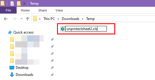
If the script doesn’t work, change its extension to XLS from XLSX .

Now, run the VBA script again, and this time Excel should be able to look up the password.

Unlock Excel Sheet Using a Workaround

Create a new Excel workbook on your device.

Now, navigate to the locked worksheet opened on another workbook. Click on any blank cell in the worksheet and press Ctrl + A to select everything.

Press Ctrl + C to copy the content.

Go to your new workbook and paste the copied data into a sheet by pressing Ctrl + V .

This method only works if the workbook isn’t locked with a password and you’ve got read access to it.

Conclusions

These are all the tried and tested methods to unprotect an Excel sheet. It becomes easier to unlock and disable the protection of workbooks and worksheets if you know the password. For this, you should use the Unprotect Sheet feature.

However, if you can’t recall the password, you can use other methods like Google Drive , XML editing , VBA scripting , an online Excel file unlocker , etc.

Did you find the Excel tutorial helpful? Comment below. Also, if you know a better method that I might have missed, mention that in your comment.

About the Author

Subscribe for awesome Microsoft Excel videos 😃

• Pivot Table Tips and Tricks You Need to Know
• Everything You Need to Know About Excel Tables
• The Complete Guide to Power Query
• Introduction To Power Query M Code
• The Complete List of Keyboard Shortcuts in Microsoft Excel
• The Complete List of VBA Keyboard Shortcuts in Microsoft Excel

Related Posts

What is an Absolute Reference in Excel?

May 10, 2024

Wondering what is an absolute reference in Excel? Read this essential Excel...

What Does $ Mean in Excel?

May 9, 2024

What does $ mean in Excel? Read on to learn everything you need to know about...

8 Ways to Move a Row in Microsoft Excel

May 8, 2024

You're reorganizing data sets, restructuring tables, or simply adjusting the...

Submit a Comment Cancel reply

Your email address will not be published. Required fields are marked *

Save my name, email, and website in this browser for the next time I comment.

Submit Comment

This site uses Akismet to reduce spam. Learn how your comment data is processed .

Get the Latest Microsoft Excel Tips

Follow us to stay up to date with the latest in Microsoft Excel!

Excel: What are macros and what do they do

E xcel macros increase productivity and save time when creating a complex workbook or worksheet. Even if you start with some of the best Microsoft Excel templates , adding macros simplifies using your spreadsheet in the future. Here's an explanation of what Excel macros are, what you can do with a macro, how to write and record macros to customize your workbook, and how to run macros to automate and speed up repetitive tasks.

Excel macros defined

An Excel macro is a series of commands stored in a workbook. A macro can replace actions that are as simple as a few menu choices and mouse clicks. By recording your actions, you can assign macros and replay them again with a tap of a shortcut key.

More complicated macros might be a complete program written in the Visual Basic editor using VBA code. VBA stands for Visual Basic for Applications, a programming language that includes special commands specific to Excel.

When you open macro-enabled workbooks, which are Excel files with an XLSM extension, Microsoft Office alerts you with a security warning. Macros can be dangerous and contain malicious code, so use caution.

If you don't know the origin of a file or are unsure if the creator is trustworthy, don't activate the macros. If you know the file is safe and want to use the VBA macros, choose Enable Content in the security warning.

You can bypass this warning by turning on macros in Microsoft Office Trust Center settings. Make sure you understand the risks if you do so. In the File tab , select Options , then choose Trust Center .

What can I do with Excel macros?

Excel macros are helpful. You can use macros to apply formatting to cells, rows, columns, and worksheets, sort and filter information, and perform data analytics to get a workbook ready for use.

Macros can build charts, graphs, and tables for creating reports. It imports or exports the data from other sources. Excel VBA macros can also generate documents and send emails, cutting your work to a minimum.

How to create, record, and run Excel macros

How to record a macro.

In short, open the Developer tab, select the Record Macro button, and type a macro name. You can store a macro in a Personal Macro Workbook that's available from any worksheet or in This Workbook if you only want to use it on your current worksheets.

Excel records your actions. Perform the steps you want to repeat when you run the macro in the future. Click the Stop Recording button when you're done. That way, you won't add unnecessary steps.

If you don't see the Developer tab, right-click the Excel ribbon and choose Customize the Ribbon from the drop-down menu. Tick the check box for Developer . The Developer tab appears between the View and Help tabs.

How to write VBA code

If you want to learn Visual Basic for Applications, start with our guide to creating Excel macros . If you're a beginner, unfamiliar with VBA, or want to learn more about VBA for Excel, Microsoft's macro tutorial is a good resource.

If you know VBA, open the Developer tab and select Visual Basic from the toolbar to open the VBA Editor. Alternatively, press Alt + F11 to toggle back and forth between the VBA Editor and your Excel workbook.

You can assign a keyboard shortcut to Excel macros written in VBA code, just as you can with recorded macros. Since you're using macros to save time, triggering them with keystrokes is a great idea.

What platforms support Excel macros?

You can only create Excel macros on the desktop version of Excel. The desktop version of Excel is available for Windows PCs and Mac computers. While you can't make new macros in Excel online, you can run macro-enabled workbooks. The Excel mobile app cannot run macros.

You can also use Excel Online to run macros on an inexpensive and long-lasting Chromebook . However, Microsoft didn't make a desktop version for ChromeOS. If you want to record macros or create code for a spreadsheet, you'll need another solution.

More macro options

Google Sheets has macro recording and an Apps Script Editor where you can write custom code. It's hard to beat Microsoft Excel, but Google Sheets is a worthy competitor that might be able to handle most of your needs.

How to use Microsoft 365 (Office) on a Chromebook

Accessibility best practices with Excel spreadsheets

This topic gives you step-by-step instructions and best practices for making your Excel spreadsheets accessible and unlock your content to everyone, including people with disabilities.

You learn, for example, how to work with the Accessibility Checker to tackle accessibility issues while you're creating your spreadsheet. You'll also learn how to add alt texts to images so that people using screen readers are able to listen to what the image is all about. You can also read about how to create accessible tables and how to use templates, fonts, and colors to maximize the inclusiveness of your spreadsheets before sharing them with others.

In this topic

Best practices for making excel spreadsheets accessible, check accessibility while you work in excel.

Create accessible tables

Use an accessible template

Add text to cell a1, add alt text to visuals, add accessible hyperlink text and screentips, use accessible font format and color, create accessible charts.

Rename worksheets

Delete blank worksheets

Name cells and ranges, test the accessibility of your worksheets, best practices for making excel spreadsheets accessible.

The following table includes key best practices for creating Excel spreadsheets that are accessible to people with disabilities.

Top of Page

Check accessibility while you work in Excel 

The Accessibility Checker is a tool that reviews your content and flags accessibility issues it comes across. It explains why each issue might be a potential problem for someone with a disability. The Accessibility Checker also suggests how you can resolve the issues that appear.

In Excel, the Accessibility Checker runs automatically in the background when you're creating a document. If the Accessibility Checker detects accessibility issues, you will get a reminder in the status bar.

To manually launch the Accessibility Checker, select Review > Check Accessibility . The Accessibility pane and the Accessibility ribbon open, and you can now review and fix accessibility issues. The Accessibility ribbon contains all the tools you need to create accessible spreadsheets in one place. For more info, go to  Accessibility Ribbon  and  Improve accessibility with the Accessibility Checker .

Create accessible tables

Tables can help you identify a set of data by name, and you can format the table using styles that make the data stand out. When you carefully name and format your table, you can be sure that everyone can understand your data.

It is also important to specify column header information and use a simple table structure to make sure that screen reader users can navigate the tables easily. 

Name a table

By default, Excel names the tables you create as Table1, Table2, Table3, and so on. To make it easier to refer to a table, give each table a descriptive name. A meaningful table name like "EmployeeList" is more helpful than the generic "Table1." 

With the descriptive name, you can, for example, quickly jump to the table with the Go To command (Ctrl+G) or the Name Manager  dialog box. You can also easily refer to the table in formulas.

Place the cursor anywhere in the table.

On the Table Design tab, under Table Name , replace the default name, such as 'Table1,' with a more descriptive one.

Note:  Table names must start with a letter, an underscore (_), or a backslash (\) and cannot contain spaces. For more info, see section "Important notes for names" in Rename an Excel table .

Select an accessible table style

Light colored tables with low contrast can be hard to read. To make your table more accessible, select a table style that has colors with a strong contrast. For example, choose a style that alternates between white and a dark color, such as black, dark grey, or dark blue.

On the Table Design tab, in the Table Styles  group, select the style you want.

Use table headers

Screen readers use header information to identify rows and columns. Clear table headers provide context and make navigating the table content easier.

Place the cursor anywhere in a table.

On the Table Design tab, in the Table Style Options group, select the Header Row checkbox.

Type the column headings.

For instructions on how to add headers to a new table, go to Create a table .

Table structures to avoid

Design your tables keeping in mind the following:

Avoid blank cells, columns, and rows. When navigating using the keyboard, a blank cell, column, or row might lead a screen reader user to believe there is nothing more in the table.

If there is no need for a blank cell, column, or row, consider deleting it.

If you cannot avoid a blank cell, column, or row, enter text explaining that it is blank. For example, type N/A  or Intentionally Blank .

Avoid splitting or merging cells: Screen readers keep track of their location in a table by counting table cells. If a table is nested within another table or if a cell is merged or split, the screen reader loses count and can’t provide helpful information about the table after that point. Merged or split cells can make navigating Excel tables with assistive technologies very difficult, if not impossible. Always keep your tables straightforward and simple. To ensure that tables don't contain split cells, merged cells, or nested tables, use the  Accessibility Checker .

Use one of the accessible Excel templates to make sure that your spreadsheet design, colors, contrast, and fonts are accessible for all audiences. The templates are also designed so that screen readers can more easily read the spreadsheet content.

When selecting a template, look for a template that has several features that support accessibility. For example:

Using enough white space makes the spreadsheet easier to read.

Colors with contrast make them easier to tell apart for low vision and colorblind readers.

Larger fonts are easier for low-vision users.

Preset descriptive headings and labels make the spreadsheet easier to understand for users who navigate it with a screen reader.

For the step-by-step instructions on how to use accessible templates, go to Video: Start with an accessible Excel template .

A screen reader starts reading any worksheet from cell A1. If you have a table on the worksheet, A1 should preferably be the title of the table.

If the sheet is long or complex, add instructions or an overview of the sheet in cell A1. This will inform people who are blind what’s being presented in your worksheet and how to use it. This instructional text can match the background color. This will hide it from people who can see, but allows it to be read by screen readers.

Alt text helps people who can’t see the screen to understand what’s important in visual content. Visual content includes pictures, SmartArt graphics, shapes, groups, charts, pivot charts, embedded objects, ink, and videos. In alt text, briefly describe the image and mention its intent. Screen readers read the text to describe the image to users who can’t see the image.

Avoid using text in images as the sole method of conveying important information. If you must use an image with text in it, repeat that text in the document. In alt text, briefly describe the image and mention the existence of the text and its intent.

Tip:  To write a good alt text, make sure to convey the content and the purpose of the image in a concise and unambiguous manner. The alt text shouldn’t be longer than a short sentence or two—most of the time a few thoughtfully selected words will do. Do not repeat the surrounding textual content as alt text or use phrases referring to images, such as, "a graphic of" or "an image of." For more info on how to write alt text, go to Everything you need to know to write effective alt text .

For the step-by-step instructions on how to add alt text, go to Add alternative text to a shape, picture, chart, SmartArt graphic, or other object .

To find missing alt text, use the  Accessibility Checker .

Note:  For audio and video content, in addition to alt text, include closed captioning for people who are deaf or hard of hearing.

People who use screen readers sometimes scan a list of links. Links should convey clear and accurate information about the destination. For example, avoid using link texts such as "Click here," "See this page," "Go here," or "Learn more." Instead include the full title of the destination page. You can also add ScreenTips that appear when your cursor hovers over text or images that include a hyperlink.

Tip:  If the title on the hyperlink's destination page gives an accurate summary of what’s on the page, use it for the hyperlink text. For example, this hyperlink text matches the title on the destination page: Create more with Microsoft templates .

For the step-by-step instructions on how to create hyperlinks and ScreenTips, go to Work with links in Excel .

An accessible font doesn't exclude or slow down the reading speed of anyone reading a spreadsheet, including people with low vision or reading disability or people who are blind. The right font improves the legibility and readability of the spreadsheet.

For instructions on how to change the default font, go to Change the font size .

Use accessible font format

Here are some ideas to consider:

To reduce the reading load, select familiar sans serif fonts such as Arial or Calibri. Avoid using all capital letters and excessive italics or underlines.

A person with a vision disability might miss out on the meaning conveyed by particular colors. For example, add an underline to color-coded hyperlink text so that people who are colorblind know that the text is linked even if they can’t see the color.

For headings, consider adding bold or using a larger font.

Use accessible font color

The text in your spreadsheet should be readable in a high contrast mode. For example, use bright colors or high-contrast color schemes on opposite ends of the color spectrum. White and black schemes make it easier for people who are colorblind to distinguish text and shapes.

To ensure that text displays well in a high contrast mode, use the Automatic setting for font colors. For instructions on how to change the font color, go to  Format text in cells .

Use the Accessibility Checker  to analyze the spreadsheet and find insufficient color contrast. The tool now checks the documents for text color against page color, table cell backgrounds, highlight, textbox fill color, paragraph shading, shape and SmartArt fills, headers and footers, and links.

Use an accessible template .

Charts help make complex information easier to understand. To make charts accessible, use clear and descriptive language for the chart elements, such as the chart title, axis titles, and data labels. Also make sure their formatting is accessible.

For instructions on how to add chart elements to your chart and make them accessible, go to Video: Create accessible charts in Excel .

Format a chart element

Select the chart element you want to format, for example, the chart title or data labels.

Select the Format tab.

Under the Current Selection group, select Format Selection . The Format pane opens to the right.

Select the formatting options that make your chart element accessible, such as a larger font or well-contrasting colors.

Rename worksheets

Screen readers read worksheet names, so make sure those labels are clear and descriptive. Using unique names for worksheets makes it easier to navigate the workbook.

By default, Excel names worksheets as Sheet1, Sheet2, Sheet3, and so on, but you can easily rename them. For instructions on how to rename worksheets, go to Rename a worksheet .

Screen readers read worksheet names, so blank worksheets might be confusing. Do not include any blank sheets in your workbooks.

For instructions on how to delete worksheets, go to Insert or delete a worksheet .

Name cells and ranges so that screen reader users can quickly identify the purpose of cells and ranges in Excel worksheets. Users can use the Go To command (Ctrl+G) to open up a dialog box which lists all the defined names. By selecting a name, a user can quickly jump to the named location.

Select the cell or range of cells that you want to name.

Select Formulas > Define name .

Enter the name and select OK .

Note:  The name must start with a letter, an underscore (_), or a backslash (\) and cannot contain spaces.

When your spreadsheet is ready and you've run the Accessibility Checker to make sure it is inclusive, you can try navigating the spreadsheet using a screen reader, for example, Narrator. Narrator comes with Windows, so there's no need to install anything. This is one additional way to spot issues in the navigation, for example.

Start the screen reader. For example, to start Narrator, press Ctrl+Windows logo key+Enter.

Press F6 until the focus, the blue rectangle, is on the worksheet table grid.

Do the following to test your worksheets:

Use the arrow keys to move between the cells in the table grid.

To check the worksheet names in your spreadsheet, press F6 until the focus is on the name of the current worksheet, and then use the Left and Right arrow keys to hear the other worksheet names.

If your worksheet contains floating shapes such images, press Ctrl+Alt+5. Then, to cycle through the floating shapes, press the Tab key. To return to the normal navigation, press Esc.

Fix any accessibility issues you spotted when navigating with a screen reader.

Exit the screen reader. For example, to exit Narrator, press Ctrl+Windows logo key+Enter.

Note:  Also make sure that your worksheets can be easily read on a mobile phone. This not only benefits people who have low vision and use magnification, but it also benefits a very broad set of mobile phone users.

Rules for the Accessibility Checker

Everything you need to know to write effective alt text

Make your Word documents accessible to people with disabilities

Make your PowerPoint presentations accessible to people with disabilities

Make your Outlook email accessible to people with disabilities

Make your OneNote notebooks accessible to people with disabilities

Excel help & learning

In Excel, the Accessibility Checker runs automatically in the background when you're creating a document. If the Accessibility Checker detects accessibility issues, you will get a reminder in the status bar.

To manually launch the Accessibility Checker, select Review > Check Accessibility . The Accessibility pane and the Accessibility ribbon open, and you can now review and fix accessibility issues. The Accessibility ribbon contains all the tools you need to create accessible spreadsheets in one place. For more info, go to Accessibility Ribbon and Improve accessibility with the Accessibility Checker .

Tables can help you identify a set of data by name, and you can format the table using styles that make the data stand out. When you carefully name and format your table, you can be sure that everyone can understand your data.

It is also important to specify column header information and use a simple table structure to make sure that screen reader users can navigate the tables easily.

By default, Excel names the tables you create as Table1, Table2, Table3, and so on. To make it easier to refer to a table, give each table a descriptive name. A meaningful table name like "EmployeeList" is more helpful than the generic "Table1."

With the descriptive name, you can, for example, quickly jump to the table with the Go To command (Control+G) or the Name Manager dialog box. You can also easily refer to the table in formulas.

On the Table  tab, under Table Name , replace the default name, such as 'Table1,' with a more descriptive one.

Note:  Table names must start with a letter, an underscore (_), or a backslash (\) and cannot contain spaces. For more info, see section "Important notes for names" in Rename an Excel table .

Light colored tables with low contrast can be hard to read. To make your table more accessible, select a table style that has colors with a strong contrast. For example, choose a style that alternates between white and a dark color, such as black, dark grey, or dark blue.

On the Table  tab, in the table styles group, select the style you want.

On the Table  tab, in the table styles group, select the Header Row checkbox.

Avoid blank cells, columns, and rows. When navigating using the keyboard, a blank cell, column, or row might lead a screen reader user to believe there is nothing more in the table.

If there is no need for a blank cell, column, or row, consider deleting it.

If you cannot avoid a blank cell, column, or row, enter text explaining that it is blank. For example, type N/A or Intentionally Blank .

Avoid splitting or merging cells: Screen readers keep track of their location in a table by counting table cells. If a table is nested within another table or if a cell is merged or split, the screen reader loses count and can’t provide helpful information about the table after that point. Merged or split cells can make navigating Excel tables with assistive technologies very difficult, if not impossible. Always keep your tables straightforward and simple. To ensure that tables don't contain split cells, merged cells, or nested tables, use the Accessibility Checker .

Use one of the accessible Excel templates to make sure that your spreadsheet design, colors, contrast, and fonts are accessible for all audiences. The templates are also designed so that screen readers can more easily read the spreadsheet content.

When selecting a template, look for a template that has several features that support accessibility. For example:

Using enough white space makes the spreadsheet easier to read.

Colors with contrast make them easier to tell apart for low vision and colorblind readers.

To find an accessible template, select File > New from Template .

In the Search text field, type accessible templates and press Return.

In the search results, select a suitable template.

To find missing alt text, use the Accessibility Checker .

Note:  For audio and video content, in addition to alt text, include closed captioning for people who are deaf or hard of hearing.

For the step-by-step instructions on how to create hyperlinks and ScreenTips, go to  Create or edit a hyperlink .

For instructions on how to change the default font, go to Change the default font in Excel for Mac .

Use accessible font format

Use accessible font color.

To ensure that text displays well in a high contrast mode, use the Automatic setting for font colors. For instructions on how to change the font color, go to Format text in cells .

Use the Accessibility Checker to analyze the spreadsheet and find insufficient color contrast. The tool now checks the documents for text color against page color, table cell backgrounds, highlight, textbox fill color, paragraph shading, shape and SmartArt fills, headers and footers, and links.

Charts help make complex information easier to understand. To make charts accessible, use clear and descriptive language for the chart elements, such as the chart title, axis titles, and data labels. Also make sure their formatting is accessible.

For instructions on how to add chart elements to your chart and make them accessible, go to Create a chart in Excel for Mac  and  Video: Create accessible charts in Excel .

Select the chart element you want to format, for example, the chart title or data labels.

Select Format Pane . The pane opens to the right.

Select the formatting options that make your chart element accessible, such as well-contrasting colors.

Screen readers read worksheet names, so make sure those labels are clear and descriptive. Using unique names for worksheets makes it easier to navigate the workbook.

By default, Excel names worksheets as Sheet1, Sheet2, Sheet3, and so on, but you can easily rename them.

Do one of the following:

Double-click the sheet tab, and type the new name.

On the Home tab, select Format > Rename Sheet , and type the new name.

Screen readers read worksheet names, so blank worksheets might be confusing. Do not include any blank sheets in your workbooks.

Go to the worksheet you want to delete.

On the Home tab, select Delete > Delete Sheet , and then select Delete to confirm the deletion.

Name cells and ranges so that screen reader users can quickly identify the purpose of cells and ranges in Excel worksheets. Users can use the Go To command (Control+G) to open up a dialog box which lists all the defined names. By selecting a name, a user can quickly jump to the named location.

When your spreadsheet is ready and you've run the Accessibility Checker to make sure it is inclusive, you can try navigating the spreadsheet using VoiceOver, the built-in macOS screen reader. This is one additional way to spot issues in the navigation, for example.

To start VoiceOver, do one of the following:

Press Command+F5.

On the Apple menu, select System Preferences . Select Accessibility > VoiceOver , and then select the Enable VoiceOver checkbox.

Put the focus to the worksheet table grid.

To check the worksheet names in your spreadsheet, press Option+Right or Left arrow key to go to the next or previous worksheet and to hear its name. Check also that there are no blank sheets.

To check that you have defined a descriptive and useful name for all tables and important cells in your worksheet, press Control+G and review the list in the  Go To dialog box.

To exit VoiceOver, do one of the following:

On the Apple menu, select System Preferences . Select Accessibility > VoiceOver , and then clear the Enable VoiceOver checkbox.

Note:  Also make sure that your worksheets can be easily read on a mobile phone. This not only benefits people who have low vision and use magnification, but it also benefits a very broad set of mobile phone users.

Add accessible hyperlink text

With the descriptive name, you can, for example, easily refer to the table in formulas. When table names are used, you can also quickly jump to the table with the Go To command in the Excel desktop app.

Tap the default table name, and replace it with a descriptive name.

Open the tab menu and select the Table tab.

Select Table Styles , and then select the style you want.

Add headers to an existing table

Select Style Options , and then select Header Row .

Add headers to a new table

Select the cells you want to include in the table.

Open the tab menu and select the Insert tab.

Select Table .

Turn on the Table has headers switch.

Avoid splitting or merging cells: Screen readers keep track of their location in a table by counting table cells. If a table is nested within another table or if a cell is merged or split, the screen reader loses count and can’t provide helpful information about the table after that point. Merged or split cells can make navigating Excel tables with assistive technologies very difficult, if not impossible. Always keep your tables straightforward and simple.

Alt text helps people who can’t see the screen to understand what’s important in visual content. Visual content includes pictures, shapes, groups, charts, embedded objects, ink, and videos. In alt text, briefly describe the image and mention its intent. Screen readers read the text to describe the image to users who can’t see the image.

Select the visual.

Select Alt Text .

Type the alt text in the Description field.

Select Done .

People who use screen readers sometimes scan a list of links. Links should convey clear and accurate information about the destination. For example, avoid using link texts such as "Click here," "See this page," "Go here," or "Learn more." Instead include the full title of the destination page.

Go to the cell where you want to add a hyperlink.

Select Link .

In the ADDRESS  field, type the destination URL.

In the DISPLAY  field, type the text that you want to display as the link text.

Select the cells you want to format.

Open the tab menu and select the Home tab.

Select the current font type to open the font menu, and then select the font type you want or adjust the font size to your liking.

Select Font Color , and then pick the font color you want.

Select the chart element you want to format, for example, the chart title.

Select the formatting options that make your chart element accessible, such as a larger font or well-contrasting colors.

Tap a sheet tab, and then select Rename .

Type a brief, unique name for the sheet.

Tap a sheet tab.

Swipe left in the context menu, and then select Delete Sheet .

Select Delete to confirm the deletion.

When your spreadsheet is ready, you can try a few things to make sure it is accessible:

Switch to the full desktop or web version of Excel, and then run the Accessibility Checker. The Accessibility Checker is a tool that reviews your content and flags accessibility issues it comes across. It explains why each issue might be a potential problem for someone with a disability. The Accessibility Checker also suggests how you can resolve the issues that appear. For instructions, go to Improve accessibility with the Accessibility Checker .

In the Excel for iOS app, you can try navigating the pages using the built-in screen reader, VoiceOver.

To turn on VoiceOver, select Settings > Accessibility > VoiceOver , and then turn on the VoiceOver  switch.

To navigate the content on the spreadsheet, swipe left or right.

With the descriptive name, you can, for example, easily refer to the table in formulas. When table names are used, you can also quickly jump to the table with the Go To command in the Excel desktop app.

Select  Table Styles , and then select the style you want.

Select the Header Row option.

Tip:  When the option is selected, it’s gray.

Open the tab menu and select the  Insert  tab.

Select the Table has headers checkbox.

Alt text helps people who can’t see the screen to understand what’s important in visual content. Visual content includes pictures, graphics, shapes, groups, charts, embedded objects, ink, and videos. In alt text, briefly describe the image and mention its intent. Screen readers read the text to describe the image to users who can’t see the image.

Type a description.

Select Link , and then select Insert Link .

In the Text to display field, type the text that you want to display as the link text.

In the Address field, type the destination URL.

Select Insert .

Open the tab menu and select the  Home  tab.

From the context menu, select the Edit Text .

Tap and hold a sheet tab, and then select Rename .

Tap and hold a sheet tab, and then select Delete Sheet .

In the Excel for Android app, you can try navigating the pages using the built-in screen reader, TalkBack.

To turn on Talkback, select Settings > Accessibility > TalkBack , and then turn on the Use service switch.

Best practices for making Excel for the web spreadsheets accessible

The following table includes key best practices for creating Excel for the web spreadsheets that are accessible to people with disabilities.

To launch the Accessibility Checker, select Review > Check Accessibility . The Accessibility pane opens, and you can now review and fix accessibility issues. For more info, go to Improve accessibility with the Accessibility Checker .

With the descriptive name, you can, for example, quickly jump to the table with the Go To command (Ctrl+G). You can also easily refer to the table in formulas.

Note:  Table names must start with a letter, an underscore (_), or a backslash (\) and cannot contain spaces.

For the step-by-step instruction on how to name a table, go to Rename an Excel table .

On the Table Design tab, in the Table Styles group, select the style you want.

Select the Insert tab and then Table .

If the selected range of cells contains data that you want to display as table headers, select the My table has headers checkbox.

If the selected range of cells does not contain data that you want to display as table headers, do not select the My table has headers checkbox. Excel will create a new header row above the selected cells, with the default header names ( Column1 , Column2 , and so on)

Select OK .

Replace the default header names with new, descriptive names.

In your browser, choose an accessible  Excel template .

Select Download . The template sampler is downloaded to your device.

Open the sampler in the Excel desktop app, select the template you want to use, and then select Download template .

A web page for the template opens. To open a new workbook with the selected template in Excel for the web, select Customize in Excel .

Alt text helps people who can’t see the screen to understand what’s important in visual content. Visual content includes pictures, shapes, charts, pivot charts, ink, and videos. In alt text, briefly describe the image and mention its intent. Screen readers read the text to describe the image to users who can’t see the image.

Right-click the visual, and then select Alt Text to open the Alternative Text dialog box.

In the Description text box, type 1-2 sentences to describe the visual and its context to someone who cannot see it.

Note:  We recommend only putting text in the description field and leaving the title blank. This will provide the best experience with most major screen readers including Narrator.

Tip:  To spell check and correct a word you typed, right-click the word and select from the suggested alternatives.

For the step-by-step instructions on how to create hyperlinks, go to Work with links in Excel .

For the step-by-step instructions on how to change the font style and size, go to Change the font style and size for a worksheet .

To ensure that text displays well in a high contrast mode, use the Automatic setting for font colors. For the step-by-step instructions on how to change the font color, go to Format text in cells .

For the step-by-step instructions on how to add chart elements to your chart and make them accessible, go to Add or remove titles in a chart  and  Video: Create accessible charts in Excel .

On the Chart tab, select Format . The Chart pane opens to the right, with the options available for the selected chart element.

By default, Excel names worksheets as Sheet1, Sheet2, Sheet3, and so on, but you can easily rename them. For the step-by-step instructions on how to rename worksheets, go to Rename a worksheet .

For the step-by-step instructions on how to delete worksheets, go to Insert or delete a worksheet .

When your spreadsheet is ready and you've run the Accessibility Checker to make sure it is inclusive, you can try navigating the spreadsheet using a screen reader, for example, Narrator. Narrator comes with Windows, so there's no need to install anything. This is one additional way to spot issues in the navigation, for example.

Press Ctrl+F6 until the focus, the blue rectangle, is on the worksheet table grid. Use the arrow keys to move between the cells in the table grid.

If your worksheet contains floating shapes such images, press Ctrl+F6 until the focus is on the worksheet table grid, and then press Ctrl+F6 one more time. You hear "Grid," and the focus is on one of the floating shapes. Then, to cycle through the floating shapes, press the Tab key or Shift+Tab. To return to the normal navigation, press Esc.

To check the worksheet names in your spreadsheet, press Ctrl+F6 until the focus is on the name of the current worksheet, and then use the Tab key and Shift+Tab to hear the other worksheet names.

Technical support for customers with disabilities

Microsoft wants to provide the best possible experience for all our customers. If you have a disability or questions related to accessibility, please contact the Microsoft Disability Answer Desk for technical assistance. The Disability Answer Desk support team is trained in using many popular assistive technologies and can offer assistance in English, Spanish, French, and American Sign Language. Please go to the Microsoft Disability Answer Desk site to find out the contact details for your region.

If you are a government, commercial, or enterprise user, please contact the enterprise Disability Answer Desk .

Need more help?

Want more options.

Explore subscription benefits, browse training courses, learn how to secure your device, and more.

Microsoft 365 subscription benefits

Microsoft 365 training

Microsoft security

Accessibility center

Communities help you ask and answer questions, give feedback, and hear from experts with rich knowledge.

Ask the Microsoft Community

Microsoft Tech Community

Windows Insiders

Microsoft 365 Insiders

Find solutions to common problems or get help from a support agent.

Online support

Was this information helpful?

Thank you for your feedback.

How-To Geek

Your excel spreadsheet needs a dashboard: here's how to create one.

Have your KPIs in one place.

Quick Links

Step 1: plan ahead, step 2: prepare your workbook, step 3: create your pivottables, step 4: create your first chart, step 5: repeat the process, step 6: add slicers, step 7: add more data, step 8: tidy your workbook.

Picture this—your manager has asked you for this year's key figures. You have lots of tabs in your Excel workbook, but there's so much data for you to trawl through to get what you need. The best way to get around this is to have a dashboard containing all the important information in chart form.

You might think that a dashboard showing every bit of data is the way forward, but the whole point of a dashboard is to summarize key information (such as key performance indicators, or KPIs) so you can analyze it at a glance. Once you have copied or inputted the data that will form the dashboard into your Excel worksheet, look through your data and decide what you're going to display.

At the same time, think about how you want to display each data set. Will you use pie charts or line graphs? Would a scatter graph or a pie chart work better for some of your data? Is your data going to be dynamic or static, and will this affect the type of chart you select?

It's always good to visualize how your dashboard will look and what it will contain, so you have a better idea of what you need to do for the next steps.

Before you create your dashboard, you should ensure your data is properly prepared. This will make setting up your dashboard a lot easier, guarantee that your dashboard works smoothly, and save you time down the line. In our example, we have one large table that we'll use to extract specific information into three separate charts.

Make sure you have given each sheet an appropriate name . Do this by double-clicking a tab and typing a short sheet title that makes it easier to remember what it contains.

Then, select the data in your table, including the headers, and click "Format As Table" in the Home tab on the ribbon, choosing suitable colors and designs. Make sure you also remove any blank rows in your tables.

The next step in preparing your data is to name the table . Click anywhere within your newly formatted table, and give the table a short name in the Table Name box within the Table Design tab on the ribbon. Try to keep this to one word, if possible, for easier use later on.

The final prep step is to create a dashboard tab. Click the "+" symbol next to your tabs and rename it Dashboard . You want this to be the first sheet in your workbook, so click and drag the tab to the left of all tabs.

Now that your data is prepared, you need to create tables that will feed the data to your charts. You might think that this is an unnecessary step, because you've already got your data nicely formatted into a table, but PivotTables let you manipulate your data more easily and summarize your data more quickly .

Create Your First Pivot Table Template

Click any cell in your original data table, and in the Insert tab, click PivotTable.

Fill in the dialog box with your table's name (if it's not already filled in), and make sure you select "New Worksheet" before clicking "OK."

A new tab will open with a PivotTable area, which you will update shortly.

Duplicate and Rename Your Pivot Table Tab

As you planned ahead in step 1, you'll know how many charts you will have on your dashboard. So, you want a separate PivotTable tab for each chart you will create. Rather than creating brand new PivotTables each time, hold Ctrl and drag your first PivotTable to the right to create a copy. We want three charts on our dashboard, so we'll do this twice.

Once you have the correct number of PivotTables, rename the tabs according to the data they will contain.

Amend Your First Pivot Table

Click anywhere on the first PivotTable you created, and the PivotTable Fields sidebar will open on the right.

This is where you'll choose the data to add to your table (and this will inform your charts later on). Click one of the series and drag it to the correct area below, and repeat this process for each series you want to include. In our case, as we're on the Sales Price tab, we will click and drag Employee into the Rows section and Sale Price into the Values section. You will see your PivotTable update on the left as you do this.

Format Your Pivot Table

The final step before you create your charts is to format the PivotTable, so the data will display how you want it to when you create your chart. In our example, we want to change the numbers to a currency by selecting the data and clicking the currency icon in the Home tab.

You're now ready to create your first chart.

Click anywhere in your PivotTable and head to the ribbon. In the PivotTable Analyze tab, click "PivotChart."

Then, choose a chart that presents your data in the best way, and click "OK."

You can then format your chart and change the title and field items to suit what you're looking to display.

When you're ready, select the edge of the chart and press Ctrl+C, and then go to your dashboard sheet and press Ctrl+V. Before you add the other charts, reposition and resize this first one so that your dashboard will look great. You could even add a stylish header to your dashboard tab.

Now that you have your first PivotTable and PivotChart, follow the same steps to complete your dashboard. Head to the second PivotTable tab, adjust the fields, settings, and formatting, create your table, and paste it onto your dashboard. Continue this process until you have all the charts you wanted on your dashboard, and move them around until you're happy with how it looks.

When repositioning your charts, hold down the Alt key to make them snap into a given position. This is great for lining items up when you have more than one on a worksheet.

To make your charts more interactive, add slicers . Click any of your charts, and in the PivotChart Analyze tab, click "Insert Slicer."

Select the data that you want to be changeable in your chart, and click "OK."

Reposition the resultant slicer. Then, to make your slicer tidier, right-click anywhere on the slicer, and click "Slicer Settings."

Change the settings according to what you want the slicer to show. In our case, we don't need it to show the slicer header, so we've unchecked that box. When you're done, click "OK."

You'll notice that only the chart we selected adjusts to what you choose in the slicer. So, to apply the slicer to all charts on your dashboard, right-click the slicer and click "Report Connections." Then, choose which PivotTables your slicer controls by checking the relevant boxes, and click "OK."

If you're confused by the PivotTable names, and aren't sure which one refers to which, go back to the PivotTables and rename them.

Repeat this process for each slicer, so that your whole dashboard represents all the different options you choose from all slicers.

To select more than one item in a slicer to display in your charts, hold Ctrl as you choose your options.

Because you formatted your tables properly in step 1, when you add new data to your original data table, the PivotTables will automatically pick this up. To make sure your dashboard reflects any new data you added, go back to your dashboard and click on one of your charts. Then, in the PivotChart Analyse tab, head to the Data group and click "Refresh All" under the Refresh button.

Before you share your professional workbook, take a minute to tie up the loose ends.

First, in the View tab on the ribbon, head to the Show group, and uncheck "Formula Bar," "Gridlines," and "Headings" to make your dashboard look less like an Excel sheet and more like a professional data dashboard.

Then, hide your PivotTable tabs , as they could confuse other people when they open your workbook. To do this, click one of the tabs, hold Ctrl, and then click the other tabs. Then, right-click one of the selected tabs and click "Hide."

Finally, go back to your dashboard, and in the Page Layout tab, click the drop-down arrow under Themes. Then, choose a color scheme to make all your charts and layouts match each other.

Now that you've created a fully functional and interactive dashboard, you may want to share it with others who need to see the KPIs you've identified and analyzed.

• Mastering Bookkeeping: Excel Tips and Tricks for Efficient Assignments

Mastering Bookkeeping Assignments: Unleashing Excel Tips and Tricks for Success

Embarking on a bookkeeping assignment may initially seem daunting, but fear not unlocking the potential of Excel's tips and tricks can transform the experience into a seamless and efficient endeavor. In this guide, we'll explore essential techniques designed to enhance your bookkeeping prowess and ensure precision in financial records. The power lies in your hands to solve your bookkeeping assignments effortlessly by integrating data validation, conditional formatting, PivotTables, and more. Excel is not merely a spreadsheet tool; it is your key ally in conquering complexities with confidence. Join us as we delve into a world of practical solutions, providing you with the tools needed to excel in bookkeeping tasks and elevate your financial management skills.

1. Data Validation for Error-Free Entries

Data accuracy is the cornerstone of effective bookkeeping, and Excel's Data Validation feature offers a powerful solution to mitigate errors and ensure the integrity of your entries. By setting specific criteria for each cell or range, you establish a robust foundation for error prevention.

How to Use Data Validation:

• Select the Target Range: Begin by choosing the cells or range where you want to apply data validation. This could be a column for invoice amounts, dates, or any other critical financial data.
• Navigate to the "Data" Tab: Move to the "Data" tab on the Excel ribbon. Here, you'll find the "Data Validation" option, which is your gateway to creating error-proof entries.
• Set Validation Criteria: Click on "Data Validation" and choose the type of validation criteria that suit your needs. This might involve setting numeric limits, date ranges, or creating a list of acceptable entries.
• Input Custom Messages: To guide users attempting to input data, utilize the custom input and error messages. These messages can provide helpful instructions or alerts in case of potential errors.

Implementing Data Validation not only minimizes the risk of typos and inaccuracies but also enhances the overall reliability of your bookkeeping data. This foundational step sets the stage for a more streamlined and error-free bookkeeping experience.

2. Conditional Formatting for Quick Insights

In the dynamic realm of bookkeeping, swift insights are crucial for effective decision-making. Excel's Conditional Formatting emerges as a game-changer, allowing you to visually highlight important trends, discrepancies, or overdue payments within your financial data. This feature transforms raw numbers into a visual narrative, making it easier to interpret complex datasets at a glance.

How to Apply Conditional Formatting:

• Select Your Data Range: Begin by highlighting the data range you want to analyze. This could be a column of expenses, revenue figures, or any dataset that requires quick scrutiny.
• Access the "Conditional Formatting" Option: Navigate to the "Home" tab on the Excel ribbon, where you'll find the "Conditional Formatting" option. Click on it to reveal a range of formatting possibilities.
• Choose Formatting Rules: Explore the various formatting rules available, such as data bars, color scales, or icon sets. Select the rule that best aligns with the insights you seek to uncover.
• Customize Formatting Options: Tailor the formatting options based on your preferences. Adjust colors, set value ranges, or modify icon styles to ensure the visual representation aligns with the significance of the data.

By leveraging Conditional Formatting, you empower yourself to identify patterns and outliers effortlessly. Whether it's pinpointing areas of concern or recognizing positive trends, this tool enhances your ability to make informed decisions swiftly. In the realm of bookkeeping, where every detail matters, Conditional Formatting becomes a strategic ally for efficiency and insightful financial analysis.

3. PivotTables for Dynamic Data Analysis

In the intricate landscape of bookkeeping, where data volumes can be overwhelming, Excel's PivotTables emerge as a dynamic solution for efficient data analysis. This powerful feature allows you to organize, summarize, and extract meaningful insights from extensive datasets, making it an indispensable tool for tackling complex bookkeeping assignments.

Creating PivotTables:

• Select Your Data Range: Begin by choosing the data range you want to analyze. This could include columns with transaction details, expense categories, or any other comprehensive dataset.
• Navigate to the "Insert" Tab: Head to the "Insert" tab on the Excel ribbon. Here, you'll find the "PivotTable" option, which opens up a world of possibilities for dynamic data manipulation.
• Define Rows and Columns: Drag and drop the fields into the Rows and Columns areas of the PivotTable. This step defines how your data will be structured, providing a customizable framework for analysis.
• Utilize Filters and Values: Enhance your analysis by incorporating filters and values. This allows you to focus on specific subsets of data and perform calculations, providing a deeper understanding of your financial information.

By mastering PivotTables, you empower yourself to unravel intricate financial scenarios with ease. Whether it's dissecting revenue trends, categorizing expenses, or gaining insights into the overall financial health of your business, PivotTables offer a dynamic and customizable approach to data analysis in the realm of bookkeeping.

4. Excel Formulas for Automated Calculations

Efficiency in bookkeeping is synonymous with accurate and automated calculations, and Excel's arsenal of formulas provides a robust solution. By harnessing the power of formulas, you can streamline complex calculations, reduce manual errors, and ensure the precision of your financial reports.

Example: Using the SUM Function:

• Basic Addition: The SUM function is fundamental for adding up a range of values. For instance, =SUM(A1:A10) calculates the total of values in cells A1 through A10.
• Conditional Summation with SUMIF: When dealing with specific conditions, employ the SUMIF function. For example, =SUMIF(B1:B10, ">1000", C1:C10) sums values in the range C1:C10 where the corresponding values in B1:B10 are greater than 1000.
• Lookup Values with VLOOKUP: VLOOKUP is invaluable for searching and retrieving data. With =VLOOKUP(D1, E1:F10, 2, FALSE), Excel fetches the corresponding value in the second column of the range E1:F10 based on the match in cell D1.
• Conditional Logic with IF Function: The IF function allows for conditional logic. For instance, =IF(G1>0, "Profit", "Loss") classifies the status as "Profit" if the value in G1 is positive; otherwise, it labels it as "Loss."

Mastering these formulas not only automates calculations but also lays the groundwork for more advanced financial modeling. Excel's formulas empower you to handle diverse mathematical operations, ensuring your bookkeeping assignments are not only accurate but also efficiently executed.

5. Keyboard Shortcuts to Boost Productivity

In the fast-paced world of bookkeeping, time is of the essence. Excel's extensive array of keyboard shortcuts can be your secret weapon, significantly enhancing your productivity by reducing the need for mouse clicks and menu navigation. Here's a compilation of essential keyboard shortcuts to supercharge your efficiency:

• Ctrl+ C (Copy): Duplicate cells or selected data with Ctrl +C, and paste them elsewhere using Ctrl+ V. This fundamental shortcut streamlines the copying and pasting process.
• Ctrl+ S (Save): Ensure your progress is saved regularly by pressing Ctrl +S. This quick shortcut prevents data loss and keeps your bookkeeping assignments secure.
• Ctrl+ Z (Undo): Made a mistake? Undo it swiftly with Ctrl+ Z. This shortcut is your go-to for reverting changes and maintaining accuracy in your records.
• Ctrl+ A (Select All): Select entire rows, columns, or worksheets effortlessly by pressing Ctrl +A. This shortcut is particularly useful when dealing with extensive datasets.
• Ctrl+ Home (Navigate to Start): Quickly jump to the beginning of your worksheet using Ctrl+ Home. This is handy when dealing with large datasets, ensuring efficient navigation.
• Ctrl+ Arrow Keys (Navigate Cells): Traverse through your data seamlessly using Ctrl combined with the arrow keys. This shortcut is especially useful for large tables.
• Ctrl+1 (Format Cells): Customize cell formats swiftly with Ctrl+1. This shortcut opens the Format Cells dialog, allowing you to modify fonts, alignments, and more.
• Ctrl+ F (Find): Locate specific data within your worksheet using Ctrl+ F. This shortcut opens the Find dialog, enabling you to search for values or text effortlessly.

By incorporating these keyboard shortcuts into your bookkeeping workflow, you unlock a new level of efficiency. The time saved on routine tasks can be redirected towards more strategic aspects of financial management, ensuring you stay ahead in the ever-evolving landscape of bookkeeping.

6. Named Ranges for Easy Navigation

Efficient bookkeeping hinges on seamless organization and quick accessibility of data. Excel's Named Ranges feature emerges as a powerful tool, providing a structured approach to managing your financial information. By assigning meaningful names to specific ranges within your worksheets, you not only enhance the clarity of your formulas but also simplify navigation in even the most extensive datasets.

How to Create Named Ranges:

• Select the Range: Highlight the range of cells you want to name. This could be a column of expenses, a row of transaction dates, or any specific subset of your financial data.
• Navigate to the "Formulas" Tab: Head to the "Formulas" tab on the Excel ribbon. Here, you'll find the "Define Name" option, which opens the door to creating Named Ranges.
• Define a Meaningful Name: Enter a descriptive and meaningful name for your range. This could be as straightforward as "Expenses" or as detailed as "MonthlyIncome."
• Ensure Scope and Consistency: Specify the scope of your Named Range—whether it applies to the entire workbook or a specific worksheet. Consistency in naming conventions ensures a standardized and organized approach.

By incorporating Named Ranges into your bookkeeping arsenal, you elevate your ability to manage and analyze financial data systematically. This feature not only simplifies formulas but also transforms Excel into a more user-friendly and collaborative tool, ensuring your bookkeeping processes are efficient and error-resistant.

7. Customizing Cell Formats for Clarity

Clear and well-formatted financial data is essential for effective bookkeeping. Excel's customizable cell formatting options allow you to present your data in a visually appealing and comprehensible manner. By leveraging these features, you not only enhance the clarity of your financial reports but also facilitate a more intuitive understanding of complex information.

How to Customize Cell Formats:

• Select the Cell or Range: Begin by highlighting the cells or range you want to format. This could be numerical data, dates, or any other information within your bookkeeping sheets.
• Right-Click for Formatting Options: Right-click on the selected cells and choose the "Format Cells" option from the context menu. Alternatively, you can access this feature from the "Home" tab on the Excel ribbon.
• Choose the Desired Format: The "Format Cells" dialog box offers a plethora of formatting options. Tailor the format to suit your specific needs, whether it's currency, percentage, date, or custom formatting.
• Preview and Apply: Use the preview section within the dialog box to see how your chosen format will look. Once satisfied, click "OK" to apply the selected formatting to the chosen cells.

Formatting Tips for Clarity:

• Currency Formatting: Apply currency formatting to monetary values for a professional and standardized look. Use symbols like "$" or "€" and specify the number of decimal places to enhance precision.
• Percentage Formatting: Convert decimal values into percentages for better comprehension. This is particularly useful when presenting changes in financial metrics or analyzing growth rates.
• Date Formatting: Ensure consistency in date representation. Choose a format that aligns with your regional preferences, such as "DD/MM/YYYY" or "MM/DD/YYYY," to avoid confusion.
• Custom Formatting: Tailor formats to meet specific requirements. Custom formatting allows you to create your own format patterns, enhancing the presentation of unique data types.

Customizing cell formats not only contributes to the aesthetic appeal of your bookkeeping worksheets but also serves as a practical strategy for improving data interpretation. Whether you're emphasizing key figures, aligning dates uniformly, or presenting percentages with clarity, Excel's formatting options empower you to create financial reports that are not only accurate but also visually impactful.

8. Data Consolidation for Streamlined Reports

As bookkeepers often contend with vast datasets from multiple sources, Excel's Data Consolidation feature emerges as a crucial asset for creating comprehensive and streamlined reports. This powerful tool enables you to aggregate information from various sheets or workbooks, providing a consolidated view that simplifies analysis and enhances the efficiency of your bookkeeping tasks.

Steps for Data Consolidation:

• Select Your Target Range: Begin by identifying the individual ranges or worksheets you want to consolidate. This could involve financial data from different departments, months, or projects.
• Navigate to the "Data" Tab: Head to the "Data" tab on the Excel ribbon. Here, you'll find the "Consolidate" option, which is your gateway to creating consolidated reports.
• Choose Consolidation Function: Select the type of consolidation function that suits your reporting needs. Excel offers options such as sum, average, count, and more, depending on the nature of your data.
• Indicate Source Ranges: Specify the source ranges for consolidation. This involves identifying the cells or ranges from each worksheet or workbook that contribute to the consolidated report.
• Review and Confirm: After setting up the consolidation parameters, review the preview to ensure accuracy. Click "OK" to complete the consolidation process.

Benefits of Data Consolidation:

• Holistic View of Data: Consolidating data provides a holistic view, allowing you to assess the overall financial picture by combining information from various sources.
• Time Efficiency: Streamline your reporting process by avoiding manual data entry. Data Consolidation automates the aggregation process, saving time and reducing the risk of errors.
• Flexible Analysis: Once consolidated, your data becomes more flexible for analysis. You can easily generate reports, charts, and summaries that encompass a broader scope of financial information.
• Improved Decision-Making: Enhanced visibility into consolidated data empowers better decision-making. Identify trends, anomalies, and key performance indicators more effectively with a consolidated overview.

Data Consolidation in Excel is a potent tool for bookkeepers dealing with diverse and distributed datasets. By centralizing information into a cohesive report, you not only simplify your bookkeeping tasks but also elevate the quality and accuracy of your financial analysis. This feature is especially valuable in scenarios where a comprehensive view is essential for strategic decision-making and financial planning.

Conclusion:

In conclusion, mastering your bookkeeping assignments is within reach with the strategic application of Excel tips and tricks. By incorporating data validation, conditional formatting, PivotTables, formulas, keyboard shortcuts, and named ranges into your workflow, you'll streamline your processes and elevate the accuracy of your financial records.

Solve your bookkeeping assignments effortlessly by making Excel your go-to companion. As you implement these tips, you'll not only enhance your efficiency but also gain a deeper understanding of your financial data. Excel isn't just a spreadsheet tool – it's your key to conquering the complexities of bookkeeping with confidence and precision. So, dive in, explore the functionalities, and watch as Excel transforms your bookkeeping experience.

Post a comment...

Mastering bookkeeping: excel tips and tricks for efficient assignments submit your assignment, attached files.

Excel Data Made Easy, in WPS Spreadsheet

Wps spreadsheet is a free excel editor for effortless sheet creation, editing, saving, and sharing. seamlessly process excel spreadsheets across multiple platforms with full compatibility with microsoft office. available for pc windows, mac, linux, android, and ios devices..

See How Easy to Do with WPS Spreadsheet

Friendly ui, free alternative to microsoft excel, embark on a seamless and intuitive spreadsheet journey with wps spreadsheet's user-friendly interface, carefully crafted to resemble excel., experience the familiarity and ease of navigation, empowering you to effortlessly create, edit, and format your excel spreadsheets with confidence..

Compatible with .XLS, .XLSX Files

Wps spreadsheet supports 17 file formats, including .xls, .xlsx, .xlsm, .xlt, .csv, .txt, .pdf and more., with wps spreadsheet, effortlessly maintain the integrity of your data, formulas, formatting, charts, and other elements, ensuring seamless preservation throughout your work..

File Management and Sharing, Anywhere

Wps spreadsheet effortlessly synchronizes excel files across a range of devices: pc windows, mac, linux, android, iphone, ipad, and various cloud platforms., collaborate in real-time, track edits, versions, and contributors. with wps spreadsheet, everyone stays on the same page, ensuring smooth teamwork and effective collaboration..

Jumpstart Project with Professional Templates

Access over 100,000 stunning templates in wps office to enhance your spreadsheets effortlessly., download free, editable templates to customize captivating financial reports, engaging charts, and impactful data presentations that make a lasting impression..

Popular Features of WPS Spreadsheet

You can effortlessly combine multiple cells into a single, centered cell for improved readability and visual impact. WPS Spreadsheet provides 4 easy method to format your cells and you can even utilize convenient shortcuts to quickly apply it.

See What Our Users Have to Say

Rated as Leader

Editor's Rating: Excellent

Google Play

Editor's Choice&Top Developer

WPS Office is a solid office productivity suite that provides a good alternative to Microsoft Office at zero cost!

The documents and spreadsheets are interchangeable with Word and Excel. I like the fact that every spreadsheet can be accessed from a tab.

The user interface is clean and well laid out. Seemless flow and ease of use. As good as Excel or better.

Free All-in-One Office Suite

Wps office extends beyond the spreadsheet feature for free excel document editing. additionally, it provides comprehensive features for word precessing, powerpoint presentations, and pdf documents, ensuring seamless handling of various file formats and enhancing your productivity and efficiency on pc windows, mac, linux, android and ios devices..

What Else You May Want to Know

• Yes, you can use WPS Spreadsheet for free. The free version of WPS Spreadsheet offers most features and provides free templates that meet the requirements of daily spreadsheet tasks.
• However, for access to premium templates and advanced features such as OCR (Optical Character Recognition), a premium subscription may be required. The premium subscription offers additional functionality and tools to enhance your spreadsheet experience.
• Yes, WPS Spreadsheet is designed to be user-friendly and easy to adapt to. Its interface is intuitive, resembling popular spreadsheet software like Excel, making it effortless to create, edit, and analyze data. The familiar layout and comprehensive tools ensure a smooth and straightforward user experience.
• Absolutely! You can save your spreadsheet files directly from WPS Spreadsheet to Google Drive. WPS Spreadsheet seamlessly integrates with Google Drive, allowing you to conveniently save and sync your files to the cloud storage service. This enables you to access your files from anywhere and collaborate with others efficiently.
• The main difference between WPS Spreadsheet and Microsoft Excel lies in the cost and accessibility. WPS Spreadsheet is free to use, while Microsoft Excel often requires a subscription or purchase.
• WPS Spreadsheet offers cloud integration, allowing easy storage, synchronization and collaboration through services like Google Drive.
• Additionally, WPS Spreadsheet not only supports PC Windows, Mac, Android, and iOS devices like Microsoft Excel, but also extends its compatibility to Linux, an option not covered by Microsoft Excel.
• Hot Topics:

Get start with WPS Spreadsheet to edit Excel sheets for free!